Tutorial 8: Photometric Calibration#
This tutorial demonstrates how to compute and apply photometric offsets using brutus. Photometric offsets are multiplicative corrections that account for systematic differences between observed fluxes and model predictions, arising from filter profile differences, calibration systematics, and atmospheric model limitations.
Topics Covered#
Model grids and SED generation: the magnitude coefficient format
Synthetic observations: generating test data with known offsets
PhotometricOffsetsConfig: configuring the offset computationphotometric_offsets(): recovering offsets from posterior samples
Prerequisites#
This tutorial requires the grid data file grid_mist_v9.h5 (downloaded
automatically via Pooch on first use).
# Imports and setup
import numpy as np
import matplotlib.pyplot as plt
from pathlib import Path
import warnings
warnings.filterwarnings('ignore')

# Tutorial utilities
from tutorial_utils import (
    set_plot_style,
    find_brutus_data_file,
    save_figure as save_fig_util,
    print_section
)

# brutus imports
from brutus.data import load_models
from brutus.core import get_seds
from brutus.analysis import photometric_offsets, PhotometricOffsetsConfig

set_plot_style()
plt.rcParams['figure.figsize'] = (12, 5)

plots_dir = Path('plots/tutorial_08')
plots_dir.mkdir(parents=True, exist_ok=True)

def save_figure(fig, name):
    filepath = plots_dir / f"{name}.png"
    fig.savefig(filepath, dpi=150, bbox_inches='tight')
    print(f"  Saved: {filepath}")
Section 1: Model Grid and SED Computation#
The photometric_offsets() function operates on the same model grid used by
BruteForce. Each model is stored as magnitude polynomial coefficients with
shape (n_filters, 3):
Index |
Quantity |
Description |
|---|---|---|
0 |
mag_0 |
Unreddened apparent magnitude (at reference distance) |
1 |
R_0 |
Reddening coefficient at R(V) = 0 |
2 |
dR/dR_V |
Change in reddening coefficient with R(V) |
The reddened magnitude in a given band is:
m(band) = mag_0(band) + A_V * [R_0(band) + R_V * dR(band)]
The get_seds() function applies this formula and optionally converts
magnitudes to linear flux densities. Combined with distance scaling
(F proportional to d^-2), this produces the model photometry that
photometric_offsets() compares against observations.
# Load the stellar model grid with PS1 + 2MASS filters
print_section("Loading Model Grid")

grid_file = find_brutus_data_file('grid_mist_v9.h5')

# Select the standard PS1 + 2MASS photometric system (8 filters)
filter_names = ['PS_g', 'PS_r', 'PS_i', 'PS_z', 'PS_y',
                '2MASS_J', '2MASS_H', '2MASS_Ks']
short_names = ['g', 'r', 'i', 'z', 'y', 'J', 'H', 'Ks']

models, labels, label_mask = load_models(grid_file, filters=filter_names)

n_models, n_filt, n_coeff = models.shape
print(f"Grid shape: {models.shape}")
print(f"  {n_models:,} models x {n_filt} filters x {n_coeff} coefficients")
print(f"  Filters: {', '.join(short_names)}")
print(f"\nCoefficient structure per model per filter:")
print(f"  [0] mag_0  : unreddened magnitude at reference distance")
print(f"  [1] R_0    : reddening coefficient (at R_V = 0)")
print(f"  [2] dR/dR_V: change in reddening with R(V)")

# Demonstrate SED generation for a single model
example_idx = n_models // 2
seds_mag = get_seds(models[example_idx:example_idx+1],
                    av=np.array([0.5]), rv=np.array([3.3]),
                    return_flux=False)
seds_flux = get_seds(models[example_idx:example_idx+1],
                     av=np.array([0.5]), rv=np.array([3.3]),
                     return_flux=True)

print(f"\nExample SED (model {example_idx}, A_V=0.5, R_V=3.3):")
for i in range(n_filt):
    print(f"  {short_names[i]:>2s}: mag = {seds_mag[0, i]:.3f},  "
          f"flux = {seds_flux[0, i]:.4e}")
Loading Model Grid
==================
Reading entire dataset (49 filters) once...
Extracting 8 requested filters from memory...
Grid shape: (613530, 8, 3)
  613,530 models x 8 filters x 3 coefficients
  Filters: g, r, i, z, y, J, H, Ks

Coefficient structure per model per filter:
  [0] mag_0  : unreddened magnitude at reference distance
  [1] R_0    : reddening coefficient (at R_V = 0)
  [2] dR/dR_V: change in reddening with R(V)

Example SED (model 306765, A_V=0.5, R_V=3.3):
   g: mag = 8.616,  flux = 3.5792e-04
   r: mag = 7.445,  flux = 1.0517e-03
   i: mag = 6.888,  flux = 1.7567e-03
   z: mag = 6.601,  flux = 2.2896e-03
   y: mag = 6.441,  flux = 2.6512e-03
   J: mag = 5.210,  flux = 8.2414e-03
   H: mag = 4.368,  flux = 1.7902e-02
  Ks: mag = 4.224,  flux = 2.0436e-02
Section 2: Generating Synthetic Observations with Known Offsets#
To demonstrate offset recovery, we create a controlled experiment:
Select random stellar models from the grid with realistic parameters
Compute true photometry using
get_seds()with distance scalingApply known multiplicative offsets to simulate calibration systematics
Add photometric noise to simulate realistic observations
The photometric_offsets() function returns multiplicative correction
factors (model / observed), so if we apply an offset of 1.05 to the data
(making it 5% brighter), the recovered correction should be 1/1.05 = 0.952
to bring it back to the model prediction.
# Generate synthetic observations with known offsets
print_section("Generating Synthetic Observations")

rng = np.random.default_rng(42)
n_obj = 200

# Select random models and physical parameters
true_idxs = rng.integers(0, n_models, n_obj)
true_av = rng.uniform(0.0, 1.5, n_obj)
true_rv = rng.uniform(2.8, 3.8, n_obj)
true_dist = rng.uniform(0.5, 5.0, n_obj)  # kpc

# Generate true photometry using get_seds()
true_flux = get_seds(models[true_idxs], av=true_av, rv=true_rv,
                     return_flux=True)
true_flux /= true_dist[:, None]**2  # Scale by distance

# Define known multiplicative offsets per filter
# Values > 1: observed brighter than model; < 1: observed fainter
applied_offsets = np.array([1.04, 0.97, 1.01, 0.98, 1.03, 0.99, 1.02, 0.96])

# Expected corrections: photometric_offsets returns model/observed
expected_corrections = 1.0 / applied_offsets

# Apply offsets and add noise
observed_flux = true_flux * applied_offsets[None, :]
flux_err = 0.03 * np.abs(observed_flux)  # 3% photometric errors
observed_flux = observed_flux + rng.normal(0, flux_err)
observed_flux = np.maximum(observed_flux, 1e-10)  # Ensure positive

# Observation mask: all bands observed
mask = np.ones((n_obj, n_filt), dtype=int)

print(f"Generated {n_obj} synthetic stars across {n_filt} filters")
print(f"Photometric noise: ~3% per band")
print(f"\nApplied multiplicative offsets:")
for i in range(n_filt):
    sign = "+" if applied_offsets[i] > 1 else ""
    pct = (applied_offsets[i] - 1) * 100
    print(f"  {short_names[i]:>2s}: {applied_offsets[i]:.3f}  ({sign}{pct:.1f}%)")
Generating Synthetic Observations
=================================
Generated 200 synthetic stars across 8 filters
Photometric noise: ~3% per band

Applied multiplicative offsets:
   g: 1.040  (+4.0%)
   r: 0.970  (-3.0%)
   i: 1.010  (+1.0%)
   z: 0.980  (-2.0%)
   y: 1.030  (+3.0%)
   J: 0.990  (-1.0%)
   H: 1.020  (+2.0%)
  Ks: 0.960  (-4.0%)
Section 3: Computing Photometric Offsets#
The photometric_offsets() function requires posterior samples from
fitting: model indices, extinction, reddening shape, and distances for each
star. In practice these come from BruteForce.fit() output. For this
demonstration, we construct synthetic posteriors by perturbing the known
true parameters with small Gaussian scatter.
PhotometricOffsetsConfig#
The PhotometricOffsetsConfig class controls the offset computation:
Parameter |
Default |
Description |
|---|---|---|
|
300 |
Bootstrap realizations for uncertainty |
|
4 |
Minimum observed bands for reweighted filters |
|
3 |
Minimum observed bands for non-reweighted filters |
|
|
|
|
None |
Seed for reproducibility |
Likelihood Reweighting#
An important feature (not demonstrated here) is the mask_fit parameter.
When a band was used in the original BruteForce fit, the posterior samples
are biased toward models that fit that band well. Setting mask_fit[i] = True
triggers leave-one-out reweighting that recomputes the likelihood excluding
that band to avoid circular bias. This is critical for real fitting results
but not needed for our synthetic posteriors, which are unbiased by construction.
# Create synthetic posterior samples and compute offsets
print_section("Computing Photometric Offsets")

# --- Step 1: Create synthetic posterior samples ---
# In practice, these come from BruteForce.fit() output arrays:
#   model_idx  -> idxs    (n_obj, n_samples)
#   samps_red  -> reds    (n_obj, n_samples)
#   samps_dred -> dreds   (n_obj, n_samples)
#   samps_dist -> dists   (n_obj, n_samples)

n_samp = 25  # posterior samples per star

# Perturb true parameters to simulate posterior uncertainty
idxs = np.tile(true_idxs[:, None], (1, n_samp))
reds = np.clip(rng.normal(true_av[:, None], 0.05, (n_obj, n_samp)), 0.0, 5.0)
dreds = np.clip(rng.normal(true_rv[:, None], 0.05, (n_obj, n_samp)), 2.0, 5.0)
dists = np.clip(rng.normal(true_dist[:, None], 0.1, (n_obj, n_samp)), 0.1, 20.0)

print(f"Posterior samples: {n_obj} objects x {n_samp} samples")
print(f"  A_V perturbation:  sigma ~ 0.05 mag")
print(f"  R_V perturbation:  sigma ~ 0.05")
print(f"  Dist perturbation: sigma ~ 0.1 kpc")

# --- Step 2: Configure offset computation ---
config = PhotometricOffsetsConfig(
    n_bootstrap=300,
    min_bands_used=3,
    min_bands_unused=2,
    uncertainty_method='bootstrap_iqr',
    random_seed=42,
    progress_interval=0,
)

# --- Step 3: Run photometric_offsets ---
# mask_fit=False for all bands: uniform weights (no reweighting needed
# since synthetic posteriors are unbiased by construction)
offsets, errors, n_used = photometric_offsets(
    observed_flux, flux_err, mask,
    models, idxs, reds, dreds, dists,
    mask_fit=np.zeros(n_filt, dtype=bool),
    config=config,
    verbose=True,
)

# --- Step 4: Report results ---
print(f"\n{'Band':>6}  {'Applied':>8}  {'Expected':>9}  {'Recovered':>10}  "
      f"{'Error':>7}  {'N_used':>7}")
print("  " + "-" * 56)
for i in range(n_filt):
    print(f"  {short_names[i]:>4s}  {applied_offsets[i]:>8.4f}  "
          f"{expected_corrections[i]:>9.4f}  {offsets[i]:>10.4f}  "
          f"{errors[i]:>7.4f}  {n_used[i]:>7d}")

residuals = offsets - expected_corrections
rms = np.sqrt(np.mean(residuals**2))
max_err = np.max(np.abs(residuals))
print(f"\nRecovery statistics:")
print(f"  RMS residual:     {rms:.4f} ({rms*100:.2f}%)")
print(f"  Max |residual|:   {max_err:.4f} ({max_err*100:.2f}%)")
print(f"  Mean uncertainty: {np.mean(errors):.4f} ({np.mean(errors)*100:.2f}%)")
Computing Photometric Offsets
=============================
Posterior samples: 200 objects x 25 samples
  A_V perturbation:  sigma ~ 0.05 mag
  R_V perturbation:  sigma ~ 0.05
  Dist perturbation: sigma ~ 0.1 kpc
Photometric offset computation complete.

  Band   Applied   Expected   Recovered    Error   N_used
  --------------------------------------------------------
     g    1.0400     0.9615      0.9635   0.0081      200
     r    0.9700     1.0309      1.0381   0.0096      200
     i    1.0100     0.9901      0.9894   0.0077      200
     z    0.9800     1.0204      1.0180   0.0083      200
     y    1.0300     0.9709      0.9694   0.0067      200
     J    0.9900     1.0101      1.0094   0.0078      200
     H    1.0200     0.9804      0.9825   0.0072      200
    Ks    0.9600     1.0417      1.0450   0.0069      200

Recovery statistics:
  RMS residual:     0.0031 (0.31%)
  Max |residual|:   0.0071 (0.71%)
  Mean uncertainty: 0.0078 (0.78%)
# Visualize offset recovery
fig, axes = plt.subplots(1, 2, figsize=(14, 5))

x = np.arange(n_filt)

# Left: recovered vs expected
ax = axes[0]
ax.errorbar(x - 0.12, offsets, yerr=errors, fmt='o', capsize=5,
            color='steelblue', markersize=8, label='Recovered', zorder=5)
ax.scatter(x + 0.12, expected_corrections, marker='s', s=80,
           color='#d32f2f', edgecolor='k', linewidth=0.5,
           label='Expected (1/applied)', zorder=5)
ax.axhline(1.0, color='gray', linestyle='--', alpha=0.5, label='Unity')
ax.set_xlabel('Filter')
ax.set_ylabel('Multiplicative Correction Factor')
ax.set_title('Offset Recovery: Expected vs Recovered')
ax.set_xticks(x)
ax.set_xticklabels(short_names)
ax.legend(fontsize=9)
ax.grid(True, alpha=0.3)

# Right: residuals
ax = axes[1]
ax.errorbar(x, residuals * 100, yerr=errors * 100, fmt='o', capsize=5,
            color='steelblue', markersize=8, zorder=5)
ax.axhline(0.0, color='gray', linestyle='--', alpha=0.5)
ax.fill_between([-0.5, n_filt - 0.5], -1, 1, alpha=0.1, color='green',
                label='+/- 1% band')
ax.set_xlabel('Filter')
ax.set_ylabel('Residual (%)')
ax.set_title('Recovery Residuals')
ax.set_xticks(x)
ax.set_xticklabels(short_names)
ax.set_xlim(-0.5, n_filt - 0.5)
ax.legend(fontsize=9)
ax.grid(True, alpha=0.3)

plt.suptitle('Photometric Offset Recovery Results', fontsize=13,
             fontweight='bold')
plt.tight_layout()
save_figure(fig, 'offset_recovery')
plt.show()

print(f"\nAll {n_filt} offsets recovered; RMS residual = {rms*100:.2f}%")
Saved: plots/tutorial_08/offset_recovery.png
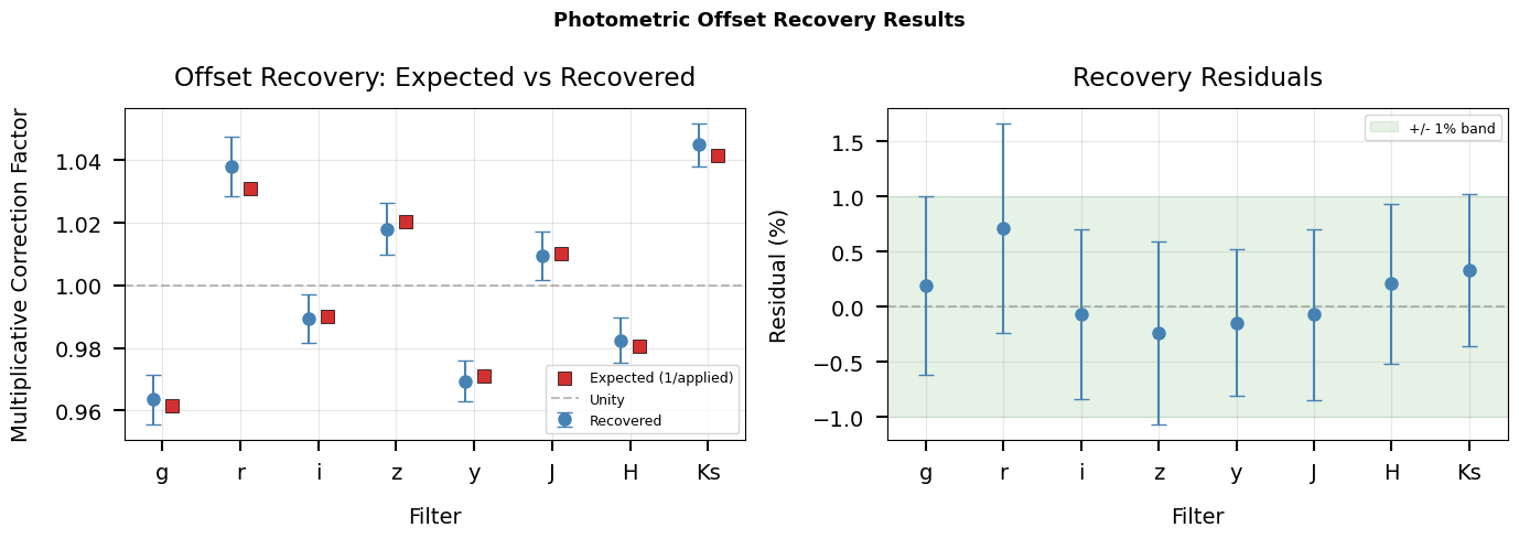
All 8 offsets recovered; RMS residual = 0.31%
Summary#
This tutorial demonstrated the complete workflow for computing photometric offsets with brutus.
Key Concepts#
Photometric offsets are multiplicative:
corrected_flux = observed_flux * offsetModel SED computation:
get_seds()applies extinction and converts to fluxPosterior samples required: offsets use
(idxs, reds, dreds, dists)from fittingBootstrap uncertainty: robust estimation via bootstrap median with IQR
The photometric_offsets() Algorithm#
Generate model SEDs for all posterior samples via
get_seds()Scale by inverse distance squared: F_model proportional to d^{-2}
Compute flux ratios: ratio = model / observed per band
For fitted bands: reweight samples via leave-one-out likelihood
Bootstrap the median ratio to get offset +/- uncertainty per filter
Practical Usage#
In a real analysis pipeline:
# After BruteForce fitting
offsets, errors, n_used = photometric_offsets(
    phot, err, mask,                      # observed data
    models, idxs, reds, dreds, dists,     # models + fit results
    mask_fit=mask_fit,                    # which bands were fitted
    config=PhotometricOffsetsConfig(),    # configuration
)
phot_corrected = phot * offsets[None, :]  # apply corrections
Next Steps#
Tutorial 9: Utility functions for photometry conversions and likelihoods
Tutorial 10: Plotting functions for visualizing fitting results
Tutorial 11: Working with BruteForce output files
print("Tutorial 8 Complete!")
print("=" * 60)
print("\nGenerated plots:")
for plot_file in sorted(plots_dir.glob('*.png')):
    print(f"  - {plot_file.name}")
print(f"\nOffset recovery ({n_filt} filters): RMS residual = {rms*100:.2f}%")
print(f"Bootstrap uncertainty: mean = {np.mean(errors)*100:.2f}%")
print(f"Objects used per filter: {n_used.min()}-{n_used.max()} of {n_obj}")
Tutorial 8 Complete!
============================================================

Generated plots:
  - offset_recovery.png

Offset recovery (8 filters): RMS residual = 0.31%
Bootstrap uncertainty: mean = 0.78%
Objects used per filter: 200-200 of 200