Tutorial 11: Working with BruteForce Results#
This tutorial covers loading, interpreting, and post-processing the HDF5 output
files produced by brutus.analysis.BruteForce. After a fit completes, the
results file contains posterior samples, best-fit statistics, and covariance
matrices for every object. Understanding how to work with these arrays is
essential for extracting science from brutus.
Topics Covered#
Loading results – HDF5 structure, keys, shapes, and dtypes
Understanding output arrays – what each dataset represents
Computing posterior summaries – medians, credible intervals, distances
Sampling from posteriors – drawing (s, A_V, R_V) realizations
Photometric conversions – flux vs magnitude representations
Visualization –
dist_vs_redandcornerplotQuality assessment – chi2/dof diagnostics and outlier flagging
Prerequisites#
This tutorial uses the pre-computed BruteForce results file
Orion_l209.1_b-19.9_mist.h5. If this file is not available, cells that
depend on it will print a skip message and continue.
# Setup: imports and plot style
import warnings

import numpy as np
import matplotlib.pyplot as plt

warnings.filterwarnings("ignore")

# Tutorial utilities
from tutorial_utils import (
    setup_tutorial,
    save_figure,
    print_section,
    find_brutus_data_file,
    load_example_results,
    assert_array_properties,
)

# Run the standardized tutorial bootstrap
info = setup_tutorial(11, title="Tutorial 11: Working with BruteForce Results")

# Matplotlib defaults for this notebook
plt.rcParams["figure.figsize"] = (10, 6)
Tutorial 11: Working with BruteForce Results
============================================

Checking data requirements for Tutorial 11
==========================================
  Found: Orion_l204.7_b-19.2_mist.h5

  All required files available
Section 1: Loading Results#
BruteForce writes its output to an HDF5 file containing several datasets.
The convenience function load_example_results() from tutorial_utils
loads all top-level datasets into a dictionary. We also demonstrate
opening the file directly with h5py to inspect its raw structure.
# ---------------------------------------------------------------
# Load pre-computed BruteForce results
# ---------------------------------------------------------------
DATA_AVAILABLE = False
results = None

try:
    results = load_example_results("Orion_l209.1_b-19.9_mist.h5")
    DATA_AVAILABLE = True
    print("Loaded BruteForce results.")
    print(f"  File: {results['filename']}")
except FileNotFoundError as exc:
    print("Results file not found -- sections that need it will be skipped.")
    print(f"  ({exc})")
Loaded BruteForce results.
  File: /mnt/c/Users/joshs/Dropbox/GitHub/brutus/tutorials/Orion_l204.7_b-19.2_mist.h5
# ---------------------------------------------------------------
# Inspect the raw HDF5 structure with h5py
# ---------------------------------------------------------------
if DATA_AVAILABLE:
    import h5py

    filepath = results["filename"]
    with h5py.File(filepath, "r") as f:
        print_section("HDF5 File Structure")
        print(f"  File: {filepath}\n")
        print(f"  {'Key':20s}  {'Shape':20s}  {'Dtype':15s}")
        print(f"  {'-'*20}  {'-'*20}  {'-'*15}")
        for key in sorted(f.keys()):
            if isinstance(f[key], h5py.Dataset):
                ds = f[key]
                print(f"  {key:20s}  {str(ds.shape):20s}  {str(ds.dtype):15s}")
            elif isinstance(f[key], h5py.Group):
                print(f"  {key:20s}  [GROUP]")
                for subkey in f[key].keys():
                    ds = f[key][subkey]
                    if isinstance(ds, h5py.Dataset):
                        print(
                            f"    {key}/{subkey:16s}  "
                            f"{str(ds.shape):20s}  {str(ds.dtype):15s}"
                        )

    # Also list the keys loaded into the results dict
    print("\nKeys in results dict:")
    for key in sorted(results):
        if key == "filename":
            continue
        val = results[key]
        if isinstance(val, np.ndarray):
            print(f"  {key:20s}  shape={str(val.shape):20s}  dtype={val.dtype}")
        elif isinstance(val, dict):
            print(f"  {key:20s}  [dict with {len(val)} sub-keys]")
else:
    print("SKIPPED -- results file not available.")
HDF5 File Structure
===================
  File: /mnt/c/Users/joshs/Dropbox/GitHub/brutus/tutorials/Orion_l204.7_b-19.2_mist.h5

  Key                   Shape                 Dtype
  --------------------  --------------------  ---------------
  labels                (50,)                 uint64
  ml_av                 (50, 250)             float32
  ml_cov_sar            (50, 250, 3, 3)       float32
  ml_rv                 (50, 250)             float32
  ml_scale              (50, 250)             float32
  model_idx             (50, 250)             int32
  obj_Nbands            (50,)                 int16
  obj_chi2min           (50,)                 float32
  obj_log_evid          (50,)                 float32
  obj_log_post          (50, 250)             float32
  samps_dist            (50, 250)             float32
  samps_dred            (50, 250)             float32
  samps_logp            (50, 250)             float32
  samps_red             (50, 250)             float32

Keys in results dict:
  labels                shape=(50,)                 dtype=uint64
  ml_av                 shape=(50, 250)             dtype=float32
  ml_cov_sar            shape=(50, 250, 3, 3)       dtype=float32
  ml_rv                 shape=(50, 250)             dtype=float32
  ml_scale              shape=(50, 250)             dtype=float32
  model_idx             shape=(50, 250)             dtype=int32
  obj_Nbands            shape=(50,)                 dtype=int16
  obj_chi2min           shape=(50,)                 dtype=float32
  obj_log_evid          shape=(50,)                 dtype=float32
  obj_log_post          shape=(50, 250)             dtype=float32
  samps_dist            shape=(50, 250)             dtype=float32
  samps_dred            shape=(50, 250)             dtype=float32
  samps_logp            shape=(50, 250)             dtype=float32
  samps_red             shape=(50, 250)             dtype=float32
Section 2: Understanding Output Arrays#
The main datasets stored in a BruteForce results file are:
Per-sample arrays (shape (Nobj, Ndraws))#
Dataset |
Description |
|---|---|
|
Model grid index for each posterior sample |
|
Maximum-likelihood distance scale factor |
|
Maximum-likelihood extinction |
|
Maximum-likelihood reddening curve shape |
|
Local covariance matrix for |
|
Log-posterior value for each draw |
Pre-computed distance/reddening draws (shape (Nobj, Ndraws))#
These are generated by draw_sar internally during the fit:
Dataset |
Description |
|---|---|
|
Posterior distance samples (kpc) |
|
Posterior reddening |
|
Posterior differential reddening |
|
Log-weights for the distance/reddening samples |
Per-object summary arrays (shape (Nobj,))#
Dataset |
Description |
|---|---|
|
Minimum chi-squared across all models |
|
Number of photometric bands used |
|
Log-evidence (marginal likelihood) |
|
Object labels from input data |
The scale factor s relates to physical distance as
$d_{\rm kpc} = 1 / \sqrt{s}$, i.e. s = 1 / d_kpc**2.
The pre-computed samps_dist array already stores distances in kpc,
so in most workflows you can use it directly rather than converting from
ml_scale.
The covariance matrix ml_cov_sar captures the local curvature of the
likelihood surface around the ML (s, A_V, R_V) for each model sample.
This is used by draw_sar to generate Monte Carlo realizations from
the posterior.
print_section("Section 2: Output Array Summary")

if not DATA_AVAILABLE:
    print("SKIPPED -- results file not available.")
else:
    # Determine number of objects and samples
    Nobj = results["ml_scale"].shape[0]
    Ndraws = results["ml_scale"].shape[1]
    print(f"Number of objects  : {Nobj}")
    print(f"Draws per object   : {Ndraws}")

    # Print summary for per-sample ML arrays
    print("\n--- ml_scale (distance scale s = 1/d_pc^2) ---")
    print(f"  shape: {results['ml_scale'].shape}")
    print(f"  min: {np.nanmin(results['ml_scale']):.4e}")
    print(f"  median: {np.nanmedian(results['ml_scale']):.4e}")
    print(f"  max: {np.nanmax(results['ml_scale']):.4e}")

    print("\n--- ml_av (ML extinction A_V in mag) ---")
    print(f"  shape: {results['ml_av'].shape}")
    print(f"  min: {np.nanmin(results['ml_av']):.3f}")
    print(f"  median: {np.nanmedian(results['ml_av']):.3f}")
    print(f"  max: {np.nanmax(results['ml_av']):.3f}")

    print("\n--- ml_rv (ML reddening curve R_V) ---")
    print(f"  shape: {results['ml_rv'].shape}")
    print(f"  min: {np.nanmin(results['ml_rv']):.3f}")
    print(f"  median: {np.nanmedian(results['ml_rv']):.3f}")
    print(f"  max: {np.nanmax(results['ml_rv']):.3f}")

    print("\n--- ml_cov_sar (covariance matrices) ---")
    print(f"  shape: {results['ml_cov_sar'].shape}")

    # Pre-computed distance/reddening draws
    print("\n--- samps_dist (posterior distance in kpc) ---")
    print(f"  shape: {results['samps_dist'].shape}")
    print(f"  min: {np.nanmin(results['samps_dist']):.3f}")
    print(f"  median: {np.nanmedian(results['samps_dist']):.3f}")
    print(f"  max: {np.nanmax(results['samps_dist']):.3f}")

    print("\n--- samps_red (posterior A_V in mag) ---")
    print(f"  shape: {results['samps_red'].shape}")
    print(f"  min: {np.nanmin(results['samps_red']):.3f}")
    print(f"  median: {np.nanmedian(results['samps_red']):.3f}")
    print(f"  max: {np.nanmax(results['samps_red']):.3f}")

    # Per-object summary arrays
    print("\n--- obj_chi2min (minimum chi-squared) ---")
    print(f"  shape: {results['obj_chi2min'].shape}")
    print(f"  min: {np.nanmin(results['obj_chi2min']):.2f}")
    print(f"  median: {np.nanmedian(results['obj_chi2min']):.2f}")
    print(f"  max: {np.nanmax(results['obj_chi2min']):.2f}")

    print("\n--- obj_Nbands (number of bands used) ---")
    print(f"  shape: {results['obj_Nbands'].shape}")
    unique_nb = np.unique(results["obj_Nbands"])
    print(f"  unique values: {unique_nb}")

    print("\n--- obj_log_evid (log-evidence) ---")
    print(f"  shape: {results['obj_log_evid'].shape}")
    finite_lnz = results["obj_log_evid"][np.isfinite(results["obj_log_evid"])]
    if len(finite_lnz) > 0:
        print(f"  min: {np.min(finite_lnz):.2f}")
        print(f"  median: {np.median(finite_lnz):.2f}")
        print(f"  max: {np.max(finite_lnz):.2f}")
    else:
        print("  (all non-finite)")

    # Verify array properties
    assert_array_properties(
        results["ml_scale"], name="ml_scale", ndim=2, shape=(Nobj, Ndraws)
    )
    assert_array_properties(
        results["ml_av"], name="ml_av", ndim=2, shape=(Nobj, Ndraws)
    )
    assert_array_properties(
        results["ml_rv"], name="ml_rv", ndim=2, shape=(Nobj, Ndraws)
    )
    assert_array_properties(
        results["ml_cov_sar"], name="ml_cov_sar", ndim=4,
        shape=(Nobj, Ndraws, 3, 3)
    )
    assert_array_properties(
        results["samps_dist"], name="samps_dist", ndim=2, shape=(Nobj, Ndraws)
    )
    assert_array_properties(
        results["obj_chi2min"], name="obj_chi2min", ndim=1, shape=(Nobj,)
    )
    assert_array_properties(
        results["obj_Nbands"], name="obj_Nbands", ndim=1, shape=(Nobj,)
    )
    print("\nAll array property checks passed.")
Section 2: Output Array Summary
===============================
Number of objects  : 50
Draws per object   : 250

--- ml_scale (distance scale s = 1/d_pc^2) ---
  shape: (50, 250)
  min: 2.8826e-04
  median: 2.9745e-01
  max: 1.5204e+01

--- ml_av (ML extinction A_V in mag) ---
  shape: (50, 250)
  min: 0.000
  median: 0.747
  max: 2.387

--- ml_rv (ML reddening curve R_V) ---
  shape: (50, 250)
  min: 2.941
  median: 3.315
  max: 4.248

--- ml_cov_sar (covariance matrices) ---
  shape: (50, 250, 3, 3)

--- samps_dist (posterior distance in kpc) ---
  shape: (50, 250)
  min: 0.253
  median: 1.838
  max: 73.391

--- samps_red (posterior A_V in mag) ---
  shape: (50, 250)
  min: 0.003
  median: 0.746
  max: 1.744

--- obj_chi2min (minimum chi-squared) ---
  shape: (50,)
  min: 0.00
  median: 1.21
  max: 113.10

--- obj_Nbands (number of bands used) ---
  shape: (50,)
  unique values: [4 5 6 7 8 9]

--- obj_log_evid (log-evidence) ---
  shape: (50,)
  min: -45.31
  median: 12.92
  max: 15.82

All array property checks passed.
Section 3: Computing Posterior Summaries#
The results file contains two ways to obtain distance posteriors:
Pre-computed samples (
samps_dist,samps_red,samps_dred): ready-to-use posterior draws generated bydraw_sarduring the fit. This is the recommended approach for most workflows.ML estimates (
ml_scale,ml_av,ml_rv): per-draw maximum-likelihood values. The scale factor relates to distance as $d_{\mathrm{kpc}} = 1/\sqrt{s}$, where $s = 1/d_{\mathrm{kpc}}^2$.
We demonstrate both approaches below and compute medians and 68%
credible intervals (16th–84th percentile) using brutus.utils.quantile.
from brutus.utils import quantile

print_section("Section 3: Posterior Summaries")

if not DATA_AVAILABLE:
    print("SKIPPED -- results file not available.")
else:
    q_levels = np.array([0.16, 0.50, 0.84])

    # --- Approach 1: Use pre-computed samps_dist / samps_red / samps_dred ---
    samps_dist = results["samps_dist"]   # kpc
    samps_red = results["samps_red"]     # A_V
    samps_dred = results["samps_dred"]   # R_V

    Nobj = samps_dist.shape[0]

    # Storage for summaries
    dist_lo = np.full(Nobj, np.nan)
    dist_med = np.full(Nobj, np.nan)
    dist_hi = np.full(Nobj, np.nan)
    av_lo = np.full(Nobj, np.nan)
    av_med = np.full(Nobj, np.nan)
    av_hi = np.full(Nobj, np.nan)
    rv_lo = np.full(Nobj, np.nan)
    rv_med = np.full(Nobj, np.nan)
    rv_hi = np.full(Nobj, np.nan)

    for i in range(Nobj):
        # Distance (already in kpc)
        d_i = samps_dist[i]
        good = np.isfinite(d_i) & (d_i > 0)
        if np.sum(good) > 1:
            q = quantile(d_i[good], q_levels)
            dist_lo[i], dist_med[i], dist_hi[i] = q

        # A_V
        av_i = samps_red[i]
        good_av = np.isfinite(av_i)
        if np.sum(good_av) > 1:
            q = quantile(av_i[good_av], q_levels)
            av_lo[i], av_med[i], av_hi[i] = q

        # R_V
        rv_i = samps_dred[i]
        good_rv = np.isfinite(rv_i)
        if np.sum(good_rv) > 1:
            q = quantile(rv_i[good_rv], q_levels)
            rv_lo[i], rv_med[i], rv_hi[i] = q

    # Print a table for the first 10 objects
    n_show = min(10, Nobj)
    print("Using pre-computed samps_dist / samps_red / samps_dred:\n")
    print(f"{'Obj':>5s}  {'d_med (kpc)':>12s}  {'d_lo':>8s}  {'d_hi':>8s}  "
          f"{'AV_med':>8s}  {'AV_lo':>8s}  {'AV_hi':>8s}  "
          f"{'RV_med':>8s}")
    print(f"{'---':>5s}  {'----------':>12s}  {'----':>8s}  {'----':>8s}  "
          f"{'------':>8s}  {'-----':>8s}  {'-----':>8s}  "
          f"{'------':>8s}")
    for i in range(n_show):
        print(
            f"{i:5d}  {dist_med[i]:12.3f}  {dist_lo[i]:8.3f}  {dist_hi[i]:8.3f}  "
            f"{av_med[i]:8.3f}  {av_lo[i]:8.3f}  {av_hi[i]:8.3f}  "
            f"{rv_med[i]:8.3f}"
        )

    print(f"\n... ({Nobj} objects total)")

    # Global summary
    valid_d = np.isfinite(dist_med)
    print(f"\nGlobal distance summary ({np.sum(valid_d)} valid objects):")
    print(f"  Median distance: {np.nanmedian(dist_med):.3f} kpc")
    print(f"  Range: [{np.nanmin(dist_med):.3f}, {np.nanmax(dist_med):.3f}] kpc")

    # --- Approach 2: Convert ml_scale manually (for reference) ---
    # Scale factor: s = 1/d_kpc^2, so d_kpc = 1/sqrt(s)
    print("\n--- Manual conversion from ml_scale (for reference) ---")
    scales = results["ml_scale"]
    s_med = np.nanmedian(scales, axis=1)
    good_s = np.isfinite(s_med) & (s_med > 0)
    d_from_scale = np.full(Nobj, np.nan)
    d_from_scale[good_s] = 1.0 / np.sqrt(s_med[good_s])  # kpc
    print(f"  Median distance from ml_scale: {np.nanmedian(d_from_scale):.3f} kpc")
    print(f"  (cf. samps_dist median: {np.nanmedian(dist_med):.3f} kpc)")
    print("  These differ because samps_dist incorporates draw_sar resampling.")
Section 3: Posterior Summaries
==============================
Using pre-computed samps_dist / samps_red / samps_dred:

  Obj   d_med (kpc)      d_lo      d_hi    AV_med     AV_lo     AV_hi    RV_med
  ---    ----------      ----      ----    ------     -----     -----    ------
    0         0.935     0.908     0.961     0.886     0.738     1.018     3.284
    1         1.695     1.585     1.809     0.816     0.688     0.938     3.208
    2         2.898     2.562     3.298     0.731     0.551     0.867     3.252
    3         2.539     2.133     2.981     0.993     0.834     1.119     3.294
    4         1.620     1.471     1.790     0.696     0.520     0.882     3.264
    5         1.399     1.282     1.568     0.986     0.816     1.155     3.361
    6         1.637     1.425     1.906     0.626     0.452     0.818     3.254
    7         1.081     1.011     1.205     1.023     0.911     1.174     3.340
    8         0.968     0.935     1.209     1.254     1.076     1.381     3.253
    9         2.120     1.878     2.360     0.718     0.572     0.900     3.291

... (50 objects total)

Global distance summary (50 valid objects):
  Median distance: 1.828 kpc
  Range: [0.271, 25.702] kpc

--- Manual conversion from ml_scale (for reference) ---
  Median distance from ml_scale: 1.826 kpc
  (cf. samps_dist median: 1.828 kpc)
  These differ because samps_dist incorporates draw_sar resampling.
# Plot a distance histogram
if DATA_AVAILABLE:
    fig, axes = plt.subplots(1, 3, figsize=(16, 5))

    # Panel 1: Distance distribution
    ax = axes[0]
    valid_d = dist_med[np.isfinite(dist_med)]
    ax.hist(valid_d, bins=40, alpha=0.7, color="steelblue", edgecolor="navy")
    ax.axvline(
        np.median(valid_d), color="red", ls="--", lw=2,
        label=f"Median = {np.median(valid_d):.2f} kpc"
    )
    ax.set_xlabel("Distance (kpc)")
    ax.set_ylabel("Number of Objects")
    ax.set_title("Distance Distribution")
    ax.legend()
    ax.grid(True, alpha=0.3)

    # Panel 2: A_V distribution
    ax = axes[1]
    valid_av = av_med[np.isfinite(av_med)]
    ax.hist(valid_av, bins=40, alpha=0.7, color="darkorange", edgecolor="brown")
    ax.axvline(
        np.median(valid_av), color="red", ls="--", lw=2,
        label=f"Median = {np.median(valid_av):.2f} mag"
    )
    ax.set_xlabel(r"$A_V$ (mag)")
    ax.set_ylabel("Number of Objects")
    ax.set_title("Extinction Distribution")
    ax.legend()
    ax.grid(True, alpha=0.3)

    # Panel 3: R_V distribution
    ax = axes[2]
    valid_rv = rv_med[np.isfinite(rv_med)]
    ax.hist(valid_rv, bins=40, alpha=0.7, color="seagreen", edgecolor="darkgreen")
    ax.axvline(
        np.median(valid_rv), color="red", ls="--", lw=2,
        label=f"Median = {np.median(valid_rv):.2f}"
    )
    ax.set_xlabel(r"$R_V$")
    ax.set_ylabel("Number of Objects")
    ax.set_title(r"$R_V$ Distribution")
    ax.legend()
    ax.grid(True, alpha=0.3)

    plt.suptitle("Posterior Summary Distributions", fontsize=14)
    save_figure(fig, 11, "posterior_summaries")
    plt.show()

    print("Histograms of median posterior values for all objects.")
else:
    print("SKIPPED -- results file not available.")
Saved: /mnt/c/Users/joshs/Dropbox/GitHub/brutus/tutorials/plots/tutorial_11/posterior_summaries.png
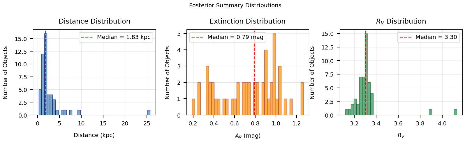
Histograms of median posterior values for all objects.
Section 4: Sampling from Posteriors#
The draw_sar function generates Monte Carlo draws from the joint
(s, A_V, R_V) posterior for a single object. It uses the per-sample
ML estimates (ml_scale, ml_av, ml_rv) and local covariance matrices
ml_cov_sar, drawing from multivariate normals and rejection-sampling
to enforce physical bounds on A_V and R_V.
This is the standard way to generate posterior realizations for downstream analysis (e.g., propagating uncertainties into derived quantities like absolute magnitude or bolometric luminosity).
Function signature#
draw_sar(scales, avs, rvs, covs_sar, ndraws=500,
         avlim=(0., 6.), rvlim=(1., 8.), rstate=None)
Returns (sdraws, adraws, rdraws) each of shape (Nsamps, ndraws).
Convert scale draws to distance via d_kpc = 1/sqrt(s).
from brutus.utils import draw_sar

print_section("Section 4: Sampling from Posteriors")

if not DATA_AVAILABLE:
    print("SKIPPED -- results file not available.")
else:
    # Pick one example object
    obj_idx = 0

    scales_obj = results["ml_scale"][obj_idx]
    avs_obj = results["ml_av"][obj_idx]
    rvs_obj = results["ml_rv"][obj_idx]
    covs_obj = results["ml_cov_sar"][obj_idx]

    print(f"Object {obj_idx}:")
    print(f"  ml_scale shape : {scales_obj.shape}")
    print(f"  ml_av shape    : {avs_obj.shape}")
    print(f"  ml_rv shape    : {rvs_obj.shape}")
    print(f"  ml_cov_sar shape: {covs_obj.shape}")

    # Draw 500 (s, A_V, R_V) realizations per sample
    ndraws = 500
    sdraws, adraws, rdraws = draw_sar(
        scales_obj, avs_obj, rvs_obj, covs_obj, ndraws=ndraws
    )

    print(f"\nDraw shapes:")
    print(f"  sdraws: {sdraws.shape}")
    print(f"  adraws: {adraws.shape}")
    print(f"  rdraws: {rdraws.shape}")

    # Flatten draws across all per-model samples
    s_flat = sdraws.ravel()
    a_flat = adraws.ravel()
    r_flat = rdraws.ravel()

    # Convert scale to distance: s = 1/d_kpc^2, so d_kpc = 1/sqrt(s)
    good = np.isfinite(s_flat) & (s_flat > 0)
    d_flat = np.full_like(s_flat, np.nan)
    d_flat[good] = 1.0 / np.sqrt(s_flat[good])  # kpc

    print(f"\nTotal draws (flattened): {len(s_flat)}")
    print(f"  Distance: median = {np.nanmedian(d_flat):.3f} kpc")
    print(f"  A_V     : median = {np.nanmedian(a_flat):.3f} mag")
    print(f"  R_V     : median = {np.nanmedian(r_flat):.3f}")

    # Compare with pre-computed samps_dist
    print(f"\nComparison with pre-computed samps_dist:")
    print(f"  samps_dist median: {np.nanmedian(results['samps_dist'][obj_idx]):.3f} kpc")
    print(f"  draw_sar median  : {np.nanmedian(d_flat):.3f} kpc")
Section 4: Sampling from Posteriors
===================================
Object 0:
  ml_scale shape : (250,)
  ml_av shape    : (250,)
  ml_rv shape    : (250,)
  ml_cov_sar shape: (250, 3, 3)

Draw shapes:
  sdraws: (250, 500)
  adraws: (250, 500)
  rdraws: (250, 500)

Total draws (flattened): 125000
  Distance: median = 0.935 kpc
  A_V     : median = 0.881 mag
  R_V     : median = 3.297

Comparison with pre-computed samps_dist:
  samps_dist median: 0.935 kpc
  draw_sar median  : 0.935 kpc
# Corner-like scatter plot of the drawn posterior samples
if DATA_AVAILABLE:
    fig, axes = plt.subplots(1, 3, figsize=(16, 5))

    # Use only finite draws
    mask_good = np.isfinite(d_flat) & np.isfinite(a_flat) & np.isfinite(r_flat)
    d_plot = d_flat[mask_good]
    a_plot = a_flat[mask_good]
    r_plot = r_flat[mask_good]

    # Panel 1: Distance vs A_V
    ax = axes[0]
    ax.scatter(d_plot, a_plot, s=1, alpha=0.15, color="steelblue")
    ax.set_xlabel("Distance (kpc)")
    ax.set_ylabel(r"$A_V$ (mag)")
    ax.set_title(r"Distance vs $A_V$")
    ax.grid(True, alpha=0.3)

    # Panel 2: Distance vs R_V
    ax = axes[1]
    ax.scatter(d_plot, r_plot, s=1, alpha=0.15, color="darkorange")
    ax.set_xlabel("Distance (kpc)")
    ax.set_ylabel(r"$R_V$")
    ax.set_title(r"Distance vs $R_V$")
    ax.grid(True, alpha=0.3)

    # Panel 3: A_V vs R_V
    ax = axes[2]
    ax.scatter(a_plot, r_plot, s=1, alpha=0.15, color="seagreen")
    ax.set_xlabel(r"$A_V$ (mag)")
    ax.set_ylabel(r"$R_V$")
    ax.set_title(r"$A_V$ vs $R_V$")
    ax.grid(True, alpha=0.3)

    plt.suptitle(
        f"Object {obj_idx}: Posterior Samples from draw_sar "
        f"({len(d_plot)} draws)",
        fontsize=14,
    )
    save_figure(fig, 11, "draw_sar_scatter")
    plt.show()

    print("Corner-like scatter of (distance, A_V, R_V) posterior draws.")
    print("Correlations between parameters are visible in the scatter patterns.")
else:
    print("SKIPPED -- results file not available.")
Saved: /mnt/c/Users/joshs/Dropbox/GitHub/brutus/tutorials/plots/tutorial_11/draw_sar_scatter.png
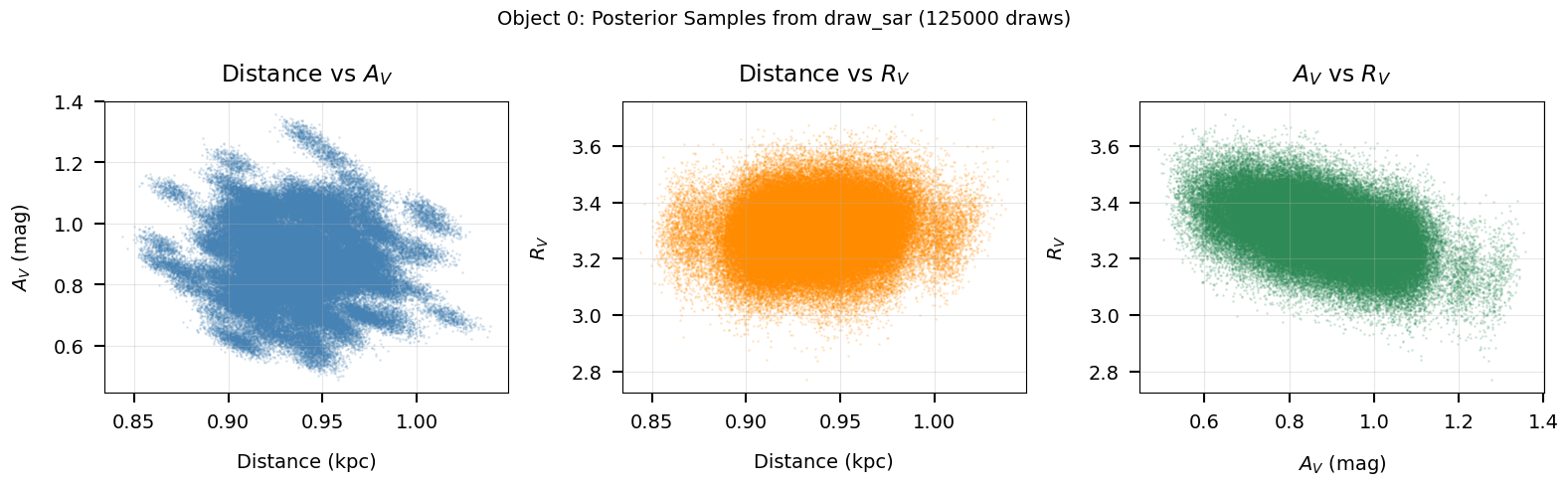
Corner-like scatter of (distance, A_V, R_V) posterior draws.
Correlations between parameters are visible in the scatter patterns.
Section 5: Photometric Conversions#
BruteForce works internally with linear flux densities (maggies),
not magnitudes. The utility functions magnitude and inv_magnitude
convert between the two representations:
$$\mathrm{flux} = 10^{-0.4 \times \mathrm{mag}}, \qquad \mathrm{mag} = -2.5 \log_{10}(\mathrm{flux})$$
This section demonstrates the round-trip conversion and, if the input photometry file is available, shows a comparison between the two representations.
from brutus.utils import magnitude, inv_magnitude

print_section("Section 5: Photometric Conversions")

# Demonstrate round-trip on synthetic data
np.random.seed(42)
mag_synth = np.random.uniform(14, 22, size=(5, 4))
magerr_synth = np.random.uniform(0.01, 0.1, size=(5, 4))

flux_synth, fluxerr_synth = inv_magnitude(mag_synth, magerr_synth)
mag_recov, magerr_recov = magnitude(flux_synth, fluxerr_synth)

residual = np.max(np.abs(mag_synth - mag_recov))
print(f"Round-trip mag -> flux -> mag:")
print(f"  Max |mag residual| = {residual:.2e}")
assert np.allclose(mag_synth, mag_recov, atol=1e-12), "Round-trip failed"
print("  Round-trip verified: exact to machine precision.")

# Load input photometry if available
PHOT_AVAILABLE = False
try:
    import h5py

    phot_path = find_brutus_data_file("Orion_l209.1_b-19.9.h5")
    with h5py.File(phot_path, "r") as f:
        fpix = f["photometry"]["pixel 0-0"]
        input_mag = fpix["mag"][:]
        input_magerr = fpix["err"][:]
        input_flux, input_fluxerr = inv_magnitude(input_mag, input_magerr)
        input_mask = np.isfinite(input_magerr)

    PHOT_AVAILABLE = True
    print(f"\nLoaded input photometry from {phot_path}")
    print(f"  Objects: {input_flux.shape[0]}, Filters: {input_flux.shape[1]}")
    print(f"  Example (object 0):")
    print(f"    Magnitudes: {input_mag[0]}")
    print(f"    Fluxes    : {input_flux[0]}")
except (FileNotFoundError, ImportError) as exc:
    print(f"\nInput photometry file not found (optional).")
    print(f"  ({exc})")
Section 5: Photometric Conversions
==================================
Round-trip mag -> flux -> mag:
  Max |mag residual| = 3.55e-15
  Round-trip verified: exact to machine precision.

Loaded input photometry from /mnt/c/Users/joshs/Dropbox/GitHub/brutus/tutorials/Orion_l204.7_b-19.2.h5
  Objects: 1642, Filters: 8
  Example (object 0):
    Magnitudes: [  14.774227 -999.       -999.       -999.         13.64316    12.724
   12.355      12.258   ]
    Fluxes    : [1.2311448e-06           inf           inf           inf 3.4892819e-06
 8.1357930e-06 1.1428786e-05 1.2496830e-05]
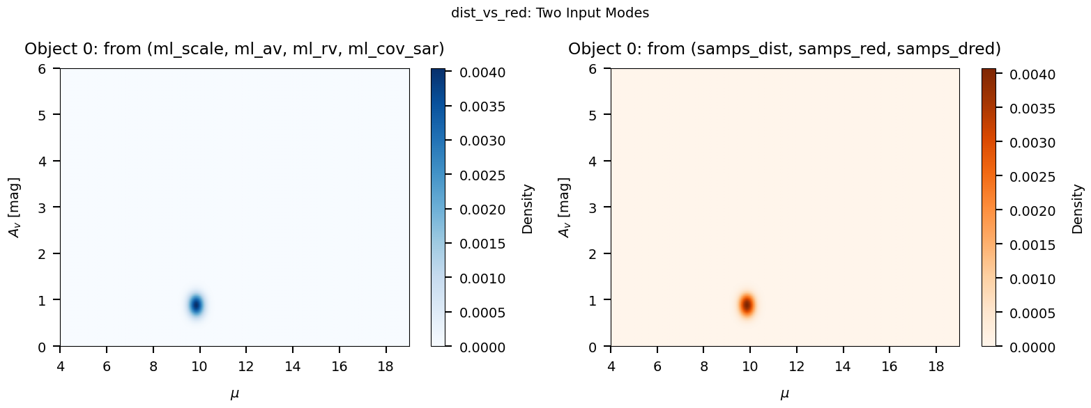
Section 6: Visualization#
The brutus.plotting module provides two key functions for visualizing
BruteForce results:
dist_vs_red: 2-D density plot of the joint distance-reddening posterior for a single object.cornerplot: Full corner plot of all stellar parameters plus (A_V, R_V, distance). Requires the model grid in memory.
Below we demonstrate dist_vs_red (which only needs the results file)
and note the requirements for cornerplot.
from brutus.plotting import dist_vs_red

print_section("Section 6: dist_vs_red Visualization")

if not DATA_AVAILABLE:
    print("SKIPPED -- results file not available.")
else:
    obj_idx = 0

    # dist_vs_red accepts either a 4-tuple (scales, avs, rvs, covs_sar)
    # or a 3-tuple (dists, reds, dreds) of pre-computed samples.
    # Here we demonstrate both approaches.

    # Approach 1: 4-tuple with ML estimates and covariances
    # (dist_vs_red will call draw_sar internally)
    data_tuple_4 = (
        results["ml_scale"][obj_idx],
        results["ml_av"][obj_idx],
        results["ml_rv"][obj_idx],
        results["ml_cov_sar"][obj_idx],
    )

    # Approach 2: 3-tuple with pre-computed distance/reddening draws
    data_tuple_3 = (
        results["samps_dist"][obj_idx],
        results["samps_red"][obj_idx],
        results["samps_dred"][obj_idx],
    )

    # Use the Orion field centre as a default coordinate
    coord = (209.1, -19.9)

    fig, axes = plt.subplots(1, 2, figsize=(16, 6))

    # Panel 1: 4-tuple (ML + covariance -> internal draw_sar)
    plt.sca(axes[0])
    try:
        H1, xe1, ye1, img1 = dist_vs_red(
            data_tuple_4,
            coord=coord,
            dist_type="distance_modulus",
            cmap="Blues",
            smooth=0.015,
            bins=300,
        )
        axes[0].set_title(f"Object {obj_idx}: from (ml_scale, ml_av, ml_rv, ml_cov_sar)")
        plt.colorbar(img1, ax=axes[0], label="Density")
    except Exception as exc:
        axes[0].text(0.5, 0.5, f"Error: {exc}", ha="center", va="center",
                     transform=axes[0].transAxes, fontsize=9)
        axes[0].set_title("4-tuple approach (failed)")

    # Panel 2: 3-tuple (pre-computed samples)
    plt.sca(axes[1])
    try:
        H2, xe2, ye2, img2 = dist_vs_red(
            data_tuple_3,
            coord=coord,
            dist_type="distance_modulus",
            cmap="Oranges",
            smooth=0.015,
            bins=300,
        )
        axes[1].set_title(f"Object {obj_idx}: from (samps_dist, samps_red, samps_dred)")
        plt.colorbar(img2, ax=axes[1], label="Density")
    except Exception as exc:
        axes[1].text(0.5, 0.5, f"Error: {exc}", ha="center", va="center",
                     transform=axes[1].transAxes, fontsize=9)
        axes[1].set_title("3-tuple approach (failed)")

    plt.suptitle("dist_vs_red: Two Input Modes", fontsize=14)
    save_figure(fig, 11, "dist_vs_red_demo")
    plt.show()

    print("Left: 4-tuple input (ml_scale, ml_av, ml_rv, ml_cov_sar).")
    print("Right: 3-tuple input (samps_dist, samps_red, samps_dred).")
    print("Both produce the same distance-reddening posterior density.")
Section 6: dist_vs_red Visualization
====================================
Saved: /mnt/c/Users/joshs/Dropbox/GitHub/brutus/tutorials/plots/tutorial_11/dist_vs_red_demo.png
Left: 4-tuple input (ml_scale, ml_av, ml_rv, ml_cov_sar).
Right: 3-tuple input (samps_dist, samps_red, samps_dred).
Both produce the same distance-reddening posterior density.
from brutus.plotting import cornerplot

print_section("Section 6b: cornerplot (reference)")

print("cornerplot requires the model grid labels array (from grid_mist_v9.h5)")
print("in addition to the results file. If you have the grid loaded, the call")
print("looks like this:")
print()
print("  fig, axes = cornerplot(")
print("      results['model_idx'][idx],")
print("      (results['ml_scale'][idx], results['ml_av'][idx],")
print("       results['ml_rv'][idx], results['ml_cov_sar'][idx]),")
print("      grid_labels,              # from load_models()")
print("      coord=(l, b),")
print("      parallax=plx,")
print("      parallax_err=plx_err,")
print("      show_titles=True,")
print("  )")
print()
print("See Tutorial 10 (Plotting Functions) for a full worked example.")
Section 6b: cornerplot (reference)
==================================
cornerplot requires the model grid labels array (from grid_mist_v9.h5)
in addition to the results file. If you have the grid loaded, the call
looks like this:

  fig, axes = cornerplot(
      results['model_idx'][idx],
      (results['ml_scale'][idx], results['ml_av'][idx],
       results['ml_rv'][idx], results['ml_cov_sar'][idx]),
      grid_labels,              # from load_models()
      coord=(l, b),
      parallax=plx,
      parallax_err=plx_err,
      show_titles=True,
  )

See Tutorial 10 (Plotting Functions) for a full worked example.
Section 7: Quality Assessment#
The primary diagnostic for BruteForce results is the p-value derived
from the chi-squared distribution. Given the best-fit obj_chi2min and
the degrees of freedom dof = Nbands - 3 (three analytically
marginalized parameters: s, A_V, R_V), we compute:
$$p = 1 - F_{\chi^2}(\chi^2_{\min};, \mathrm{dof})$$
where $F_{\chi^2}$ is the chi-squared CDF. Small p-values indicate that the observed chi-squared is improbably large under the model, flagging objects that are poorly fit (e.g., binaries, galaxies, problematic photometry).
Why not reduced chi-squared?#
While the reduced chi-squared $\chi^2_\nu = \chi^2/\mathrm{dof}$ is convenient for quick visual checks, it is not variance-stabilizing: its sampling variance is $2/\mathrm{dof}$. This means a fixed threshold like “$\chi^2_\nu > 3$” is far too lenient for objects with many bands (where $\chi^2_\nu$ concentrates tightly around 1) and overly strict for objects with few bands (where the distribution is broad). The p-value approach gives a uniform false-positive rate regardless of the number of bands, making it the principled choice for quality cuts.
Log-evidence#
The output also includes obj_log_evid, an approximate log-evidence
(marginal likelihood) computed from the grid-based Laplace
approximation. This quantity is most useful for relative model
comparison — e.g., comparing how well a MIST grid fits a given star
versus an alternative stellar model grid. Its absolute value is not
straightforwardly interpretable, so we do not use it as a standalone
quality metric here.
from scipy.stats import chi2 as chi2_dist

print_section("Section 7: Quality Assessment")

if not DATA_AVAILABLE:
    print("SKIPPED -- results file not available.")
else:
    chi2 = results["obj_chi2min"]
    Nbands = results["obj_Nbands"]

    # Degrees of freedom: 3 free parameters (s, A_V, R_V)
    n_free = 3
    dof = Nbands - n_free

    # Flag objects with insufficient bands
    insufficient = dof <= 0
    valid = ~insufficient & np.isfinite(chi2)

    print(f"Total objects          : {len(chi2)}")
    print(f"Objects with dof > 0   : {np.sum(~insufficient)}")
    print(f"Objects with dof <= 0  : {np.sum(insufficient)} (too few bands)")

    # Compute p-values from the chi-squared survival function
    pvalues = np.full(len(chi2), np.nan)
    pvalues[valid] = chi2_dist.sf(chi2[valid], dof[valid])

    if np.sum(valid) > 0:
        print(f"\nP-value summary (from chi2 CDF):")
        print(f"  Min     : {np.nanmin(pvalues[valid]):.2e}")
        print(f"  Median  : {np.nanmedian(pvalues[valid]):.3f}")
        print(f"  Max     : {np.nanmax(pvalues[valid]):.3f}")

        # Outlier flagging via p-value threshold
        p_thresh = 0.01
        outliers = valid & (pvalues < p_thresh)
        n_outliers = np.sum(outliers)
        pct_outliers = 100.0 * n_outliers / np.sum(valid)

        print(f"\nOutlier flagging (p < {p_thresh}):")
        print(f"  Flagged : {n_outliers} / {np.sum(valid)} ({pct_outliers:.1f}%)")

        good_fits = valid & (pvalues >= p_thresh)
        print(f"  Good fits: {np.sum(good_fits)} ({100.0 * np.sum(good_fits) / np.sum(valid):.1f}%)")

        # Show the flagged objects
        if n_outliers > 0:
            flagged_idx = np.where(outliers)[0]
            print(f"\n  Flagged objects:")
            print(f"  {'Obj':>5s}  {'chi2':>8s}  {'Nbands':>6s}  {'dof':>4s}  {'chi2/dof':>9s}  {'p-value':>10s}")
            for idx in flagged_idx:
                print(f"  {idx:5d}  {chi2[idx]:8.2f}  {Nbands[idx]:6d}  {dof[idx]:4d}  "
                      f"{chi2[idx]/dof[idx]:9.2f}  {pvalues[idx]:10.2e}")

        # For comparison: show why reduced chi2 thresholds are unreliable
        chi2_dof = chi2[valid] / dof[valid].astype(float)
        print(f"\nFor reference, reduced chi2 (chi2/dof) statistics:")
        print(f"  Median  : {np.median(chi2_dof):.3f}")
        print(f"  Note: The variance of chi2/dof is 2/dof, so a fixed")
        print(f"  threshold means different things at different Nbands.")

    # Log-evidence summary
    print(f"\nLog-evidence (obj_log_evid) summary:")
    lnz = results["obj_log_evid"]
    finite_lnz = lnz[np.isfinite(lnz)]
    if len(finite_lnz) > 0:
        print(f"  Min   : {np.min(finite_lnz):.2f}")
        print(f"  Median: {np.median(finite_lnz):.2f}")
        print(f"  Max   : {np.max(finite_lnz):.2f}")
        print(f"  Note: Useful for relative model comparison (e.g., MIST vs")
        print(f"  alternative grids), not as a standalone quality metric.")
    else:
        print("  (all non-finite)")
Section 7: Quality Assessment
=============================
Total objects          : 50
Objects with dof > 0   : 50
Objects with dof <= 0  : 0 (too few bands)

P-value summary (from chi2 CDF):
  Min     : 4.58e-22
  Median  : 0.739
  Max     : 0.999

Outlier flagging (p < 0.01):
  Flagged : 4 / 50 (8.0%)
  Good fits: 46 (92.0%)

  Flagged objects:
    Obj      chi2  Nbands   dof   chi2/dof     p-value
      8     10.43       5     2       5.22    5.43e-03
     39     55.47       9     6       9.25    3.72e-10
     40     82.23       9     6      13.71    1.24e-15
     44    113.10       9     6      18.85    4.58e-22

For reference, reduced chi2 (chi2/dof) statistics:
  Median  : 0.443
  Note: The variance of chi2/dof is 2/dof, so a fixed
  threshold means different things at different Nbands.

Log-evidence (obj_log_evid) summary:
  Min   : -45.31
  Median: 12.92
  Max   : 15.82
  Note: Useful for relative model comparison (e.g., MIST vs
  alternative grids), not as a standalone quality metric.
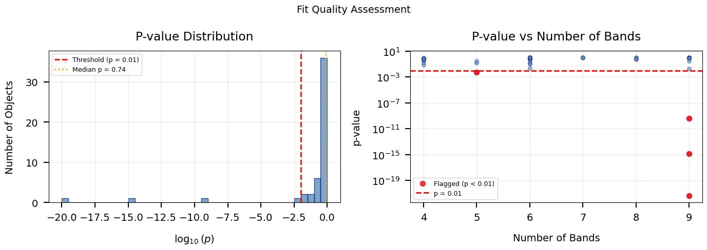
# P-value quality assessment plots
if DATA_AVAILABLE and np.sum(valid) > 0:
    fig, axes = plt.subplots(1, 2, figsize=(14, 5))

    # Panel 1: P-value histogram (log scale)
    ax = axes[0]
    pvals_plot = pvalues[valid]
    # Use log10(p) for better visualization of the distribution
    log_pvals = np.log10(np.clip(pvals_plot, 1e-20, 1.0))
    ax.hist(
        log_pvals, bins=40, alpha=0.7,
        color="steelblue", edgecolor="navy"
    )
    ax.axvline(
        np.log10(p_thresh), color="red", ls="--", lw=2,
        label=f"Threshold (p = {p_thresh})"
    )
    ax.axvline(
        np.log10(np.median(pvals_plot)), color="orange", ls=":", lw=2,
        label=f"Median p = {np.median(pvals_plot):.2f}"
    )
    ax.set_xlabel(r"$\log_{10}(p)$")
    ax.set_ylabel("Number of Objects")
    ax.set_title("P-value Distribution")
    ax.legend(fontsize=9)
    ax.grid(True, alpha=0.3)

    # Panel 2: P-value vs number of bands
    ax = axes[1]
    ax.scatter(
        Nbands[valid], pvalues[valid],
        s=30, alpha=0.6, color="steelblue", edgecolor="navy", lw=0.5
    )
    # Highlight flagged objects
    if np.sum(outliers) > 0:
        ax.scatter(
            Nbands[outliers], pvalues[outliers],
            s=60, alpha=0.8, color="red", edgecolor="darkred", lw=0.5,
            label=f"Flagged (p < {p_thresh})", zorder=5
        )
    ax.axhline(
        p_thresh, color="red", ls="--", lw=2,
        label=f"p = {p_thresh}"
    )
    ax.set_xlabel("Number of Bands")
    ax.set_ylabel("p-value")
    ax.set_yscale("log")
    ax.set_title("P-value vs Number of Bands")
    ax.legend(fontsize=9)
    ax.grid(True, alpha=0.3)

    plt.suptitle("Fit Quality Assessment", fontsize=14)
    save_figure(fig, 11, "chi2_quality")
    plt.show()

    print("Left: histogram of log10(p-value) from the chi2 CDF.")
    print("Right: p-value vs number of bands. Unlike reduced chi2, the")
    print("p-value threshold gives a uniform false-positive rate across")
    print("all band counts.")
else:
    print("SKIPPED -- results file not available or no valid chi2 values.")
Saved: /mnt/c/Users/joshs/Dropbox/GitHub/brutus/tutorials/plots/tutorial_11/chi2_quality.png
Left: histogram of log10(p-value) from the chi2 CDF.
Right: p-value vs number of bands. Unlike reduced chi2, the
p-value threshold gives a uniform false-positive rate across
all band counts.
Summary#
This tutorial demonstrated how to work with BruteForce output files:
Key Steps#
Loading – Use
load_example_results()or open directly withh5py. Inspect top-level keys, shapes, and dtypes to understand the file layout.Output arrays – Per-sample arrays (
model_idx,ml_scale,ml_av,ml_rv,ml_cov_sar), pre-computed draws (samps_dist,samps_red,samps_dred), and per-object summaries (obj_chi2min,obj_Nbands,obj_log_evid).Posterior summaries – Use
samps_dist/samps_red/samps_dredfor ready-to-use posterior samples, or convertml_scalemanually viad_kpc = 1/sqrt(s)wheres = 1/d_kpc^2. Compute quantiles withbrutus.utils.quantile.Posterior sampling –
draw_sargenerates Monte Carlo draws from the joint(s, A_V, R_V)posterior using the stored covariance matrices.Photometric conversions –
magnitudeandinv_magnitudeconvert between flux (maggies) and AB magnitudes.Visualization –
dist_vs_redshows the 2-D distance-reddening posterior (accepts either 4-tuple or 3-tuple input);cornerplotprovides a full multi-parameter view (requires the model grid).Quality assessment – Compute p-values from
obj_chi2minvia the chi-squared CDF (scipy.stats.chi2.sf). Flag objects with small p-values (e.g., p < 0.01) as poorly fit. Avoid using reduced chi-squared thresholds, which are not variance-stabilizing and behave inconsistently across different numbers of bands. The log-evidenceobj_log_evidis useful for relative model comparison but not as a standalone quality metric.