Tutorial 1: Individual Star Models#
This tutorial explores individual star modeling using EEPTracks and StarEvolTrack.
Topics Covered#
EEPTracks for parameter prediction along evolutionary tracks
StarEvolTrack for on-the-fly SED generation
Exploring parameter space (mass, metallicity, age)
Binary star modeling
Extinction and distance effects
FastNNPredictor as a lightweight alternative to StarEvolTrack
Prerequisites#
This tutorial requires the following brutus data files:
MIST_1.2_EEPtrk.h5- MIST evolutionary tracksnn_c3k.h5- Neural network for bolometric corrections
If you don’t have these files, run the optional download cell below.
# Optional: Download required data files (only needed if not already cached)
# This tutorial requires MIST evolutionary tracks and the C3K neural network.
# Uncomment the lines below to download them (~110 MB total).

# from brutus.data import fetch_tracks, fetch_nns
# fetch_tracks()    # ~60 MB  -- MIST evolutionary tracks
# fetch_nns()       # ~50 MB  -- Neural network for bolometric corrections
# Imports and setup
import numpy as np
import matplotlib.pyplot as plt
import warnings
warnings.filterwarnings('ignore')

from tutorial_utils import (
    setup_tutorial,
    find_brutus_data_file,
    save_figure as _save_fig,
    print_section,
)

info = setup_tutorial(1, title="Tutorial 01: Individual Star Models")
plots_dir = info['plot_dir']


def save_figure(fig, name):
    """Save figure to this tutorial's plot directory."""
    _save_fig(fig, 1, name)
Tutorial 01: Individual Star Models
===================================

Checking data requirements for Tutorial 1
=========================================
  Found: nn_c3k.h5
  Found: MIST_1.2_EEPtrk.h5

  All required files available
Section 1: EEPTracks - Parameter Prediction#
EEPTracks provides stellar parameter predictions along evolutionary tracks. It interpolates MIST stellar evolution models to predict physical parameters at any point along a star’s evolution.
Key Concepts#
EEP (Equivalent Evolutionary Point): A normalized coordinate along stellar evolution tracks
Tracks vs Isochrones: Tracks follow individual stars, isochrones are snapshots of populations
Parameter prediction: Get stellar properties (Teff, log g, luminosity) at any EEP
from brutus.core import EEPTracks
from brutus.data import filters

# Initialize EEPTracks
print("Loading MIST evolutionary tracks...")
mistfile = find_brutus_data_file("MIST_1.2_EEPtrk.h5")

tracks = EEPTracks(mistfile=mistfile, verbose=False)

# Explore the parameter space covered
masses = tracks.xgrid[0]  # Initial masses
metallicities = tracks.xgrid[2]  # [Fe/H] values

print(f"Loaded tracks covering {len(masses)} mass points")
print(f"  Mass range: {masses.min():.2f} - {masses.max():.2f} M☉")
print(f"  Metallicity range: {metallicities.min():.2f} - {metallicities.max():.2f}")
print(f"  Available predictions: {tracks.predictions}")
Loading MIST evolutionary tracks...
Loaded tracks covering 188 mass points
  Mass range: 0.10 - 300.00 M☉
  Metallicity range: -4.00 - 0.50
  Available predictions: [np.str_('loga'), np.str_('logl'), np.str_('logt'), np.str_('logg'), np.str_('feh_surf'), np.str_('afe_surf'), 'agewt']
# Predict parameters for a solar-mass star at different evolutionary stages
print("\nPredicting parameters for a 1 M☉ star at different evolutionary stages:\n")

# EEP ranges for different phases
eep_examples = [
    (250, "Pre-Main Sequence"),
    (350, "Zero-Age Main Sequence"),
    (400, "Middle Main Sequence"),
    (450, "Terminal-Age Main Sequence"),
    (500, "Subgiant Branch"),
    (650, "Red Giant Branch")
]

for eep, phase in eep_examples:
    try:
        # get_predictions takes [mini, eep, feh, afe]
        params = tracks.get_predictions([1.0, eep, 0.0, 0.0])

        # Extract specific parameters (indices based on tracks.predictions)
        loga_idx = tracks.predictions.index("loga")
        logl_idx = tracks.predictions.index("logl")
        logt_idx = tracks.predictions.index("logt")
        logg_idx = tracks.predictions.index("logg")

        age_gyr = 10**params[loga_idx] / 1e9
        luminosity = 10**params[logl_idx]
        teff = 10**params[logt_idx]
        logg = params[logg_idx]

        print(f"EEP {eep:3d} ({phase:25s}): Age={age_gyr:5.2f} Gyr, L={luminosity:6.2f} L☉, Teff={teff:5.0f} K, log g={logg:4.2f}")
    except:
        print(f"EEP {eep:3d} ({phase:25s}): Not available for 1 M☉ star")
Predicting parameters for a 1 M☉ star at different evolutionary stages:

EEP 250 (Pre-Main Sequence        ): Age= 0.19 Gyr, L=  0.78 L☉, Teff= 5727 K, log g=4.53
EEP 350 (Zero-Age Main Sequence   ): Age= 4.11 Gyr, L=  1.06 L☉, Teff= 5838 K, log g=4.43
EEP 400 (Middle Main Sequence     ): Age= 6.75 Gyr, L=  1.39 L☉, Teff= 5881 K, log g=4.33
EEP 450 (Terminal-Age Main Sequence): Age= 9.75 Gyr, L=  2.20 L☉, Teff= 5730 K, log g=4.08
EEP 500 (Subgiant Branch          ): Age=11.13 Gyr, L= 11.84 L☉, Teff= 4693 K, log g=3.00
EEP 650 (Red Giant Branch         ): Age=11.34 Gyr, L= 47.13 L☉, Teff= 4610 K, log g=2.35
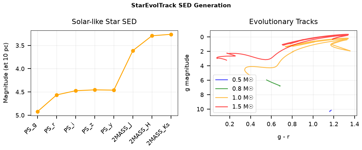
Section 2: StarEvolTrack - SED Generation#
StarEvolTrack generates SEDs using neural networks for bolometric corrections. This provides on-the-fly photometry generation at any point in parameter space.
Key Features#
Fast SED generation using neural networks
Support for any photometric filter system
Binary star modeling capabilities
Extinction and distance effects
from brutus.core import StarEvolTrack

# Set up filters (Pan-STARRS + 2MASS)
filt = filters.ps[:-2] + filters.tmass
print(f"Using filters: {', '.join(filt)}")

# Initialize StarEvolTrack
nnfile = find_brutus_data_file("nn_c3k.h5")
star = StarEvolTrack(tracks=tracks, nnfile=nnfile, filters=filt, verbose=False)

print("StarEvolTrack initialized with neural network bolometric corrections")
Using filters: PS_g, PS_r, PS_i, PS_z, PS_y, 2MASS_J, 2MASS_H, 2MASS_Ks
StarEvolTrack initialized with neural network bolometric corrections
# Generate SED for a solar-like star
print("\nGenerating SED for solar-like star (1 M☉, solar metallicity, MS):")

# Generate magnitudes at 10 pc
mags, params, _ = star.get_seds(mini=1.0, feh=0.0, eep=350, dist=10.0)

print(f"\nMagnitudes at 10 pc:")
for i, (f, m) in enumerate(zip(filt, mags)):
    print(f"  {f:10s}: {m:6.3f} mag")

# Calculate some colors
g_idx = filters.ps.index('PS_g')
r_idx = filters.ps.index('PS_r')
i_idx = filters.ps.index('PS_i')

print(f"\nColors:")
print(f"  g - r = {mags[g_idx] - mags[r_idx]:.3f}")
print(f"  r - i = {mags[r_idx] - mags[i_idx]:.3f}")
Generating SED for solar-like star (1 M☉, solar metallicity, MS):

Magnitudes at 10 pc:
  PS_g      :  4.921 mag
  PS_r      :  4.564 mag
  PS_i      :  4.473 mag
  PS_z      :  4.455 mag
  PS_y      :  4.461 mag
  2MASS_J   :  3.611 mag
  2MASS_H   :  3.293 mag
  2MASS_Ks  :  3.261 mag

Colors:
  g - r = 0.358
  r - i = 0.090
Saved: /home/user/brutus/tutorials/plots/tutorial_01/sed_generation.png
Section 3: Stellar Evolution Along Tracks#
Let’s explore how stellar parameters evolve along evolutionary tracks, from pre-main sequence through the giant branch.
# Use Gaia filters for the HRD
filt_gaia = filters.gaia
star_gaia = StarEvolTrack(tracks=tracks, nnfile=nnfile, filters=filt_gaia, verbose=False)

# Define EEP ranges for different evolutionary phases
eep_phases = {
    "Pre-MS": (202, 353),
    "MS": (353, 454),
    "SGB": (454, 605),
    "RGB": (605, 707),
    "HB/AGB": (707, 808),
}

print("EEP ranges for evolutionary phases:")
for phase, (eep_min, eep_max) in eep_phases.items():
    print(f"  {phase:8s}: EEP {eep_min:3d} - {eep_max:3d}")
EEP ranges for evolutionary phases:
  Pre-MS  : EEP 202 - 353
  MS      : EEP 353 - 454
  SGB     : EEP 454 - 605
  RGB     : EEP 605 - 707
  HB/AGB  : EEP 707 - 808
Saved: /home/user/brutus/tutorials/plots/tutorial_01/stellar_evolution.png
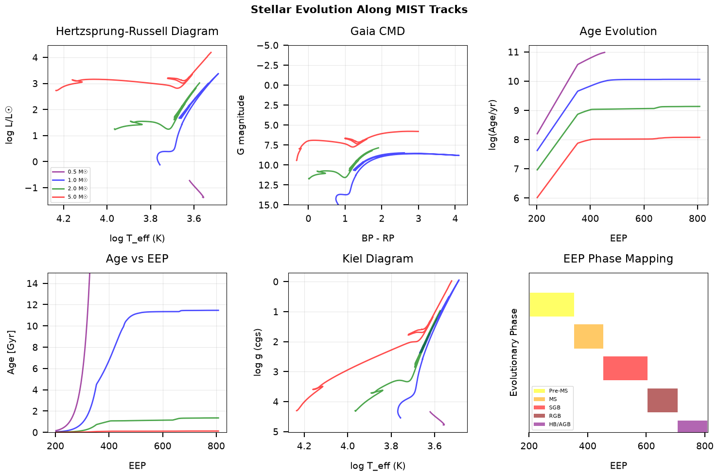
Generated stellar evolution plots showing:
  - HRD evolution for different masses
  - Position in Gaia CMD
  - Age evolution
  - Mapping of EEP to evolutionary phases
Section 4: Metallicity Effects#
Metallicity significantly affects stellar evolution and photometry. Let’s explore how [Fe/H] changes stellar properties and colors.
Saved: /home/user/brutus/tutorials/plots/tutorial_01/metallicity_effects.png
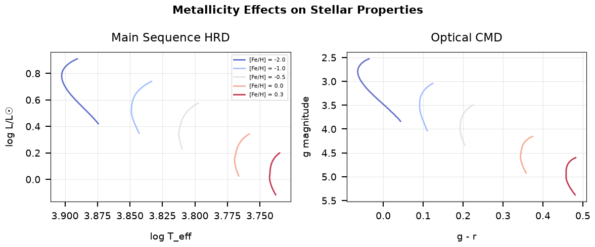
Metallicity effects demonstrated:
  - Metal-poor stars are bluer and hotter
  - MS turnoff age depends on metallicity
  - Color-metallicity relations for calibration
Section 5: Binary Star Modeling#
Unresolved binaries significantly affect observed photometry. StarEvolTrack can model binary systems using the secondary mass fraction (SMF).
Binary Parameters#
SMF (Secondary Mass Fraction): q = M₂/M₁ where M₁ is the primary mass
Equal-age assumption: Both stars have the same age and metallicity
Combined light: Total flux is the sum of both components
# Set up for binary modeling
filt_binary = filters.gaia + filters.ps[:3]  # Gaia + PS optical
star_binary = StarEvolTrack(tracks=tracks, nnfile=nnfile, filters=filt_binary, verbose=False)

# Binary parameters to explore
primary_mass = 1.0  # Solar mass primary
smf_values = [0.0, 0.3, 0.5, 0.7, 1.0]  # Single to equal-mass binary
colors_smf = ['blue', 'cyan', 'green', 'orange', 'red']

print("Binary mass ratios to explore:")
for smf in smf_values:
    secondary_mass = primary_mass * smf
    print(f"  q = {smf:.1f}: M₁ = {primary_mass:.1f} M☉, M₂ = {secondary_mass:.1f} M☉")
Binary mass ratios to explore:
  q = 0.0: M₁ = 1.0 M☉, M₂ = 0.0 M☉
  q = 0.3: M₁ = 1.0 M☉, M₂ = 0.3 M☉
  q = 0.5: M₁ = 1.0 M☉, M₂ = 0.5 M☉
  q = 0.7: M₁ = 1.0 M☉, M₂ = 0.7 M☉
  q = 1.0: M₁ = 1.0 M☉, M₂ = 1.0 M☉
Saved: /home/user/brutus/tutorials/plots/tutorial_01/binary_modeling.png
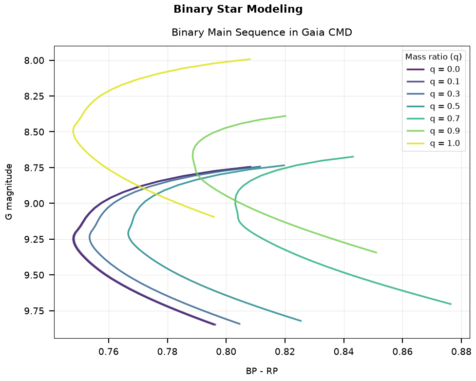
Binary modeling demonstrated:
  - Binaries shift stars above the MS
  - Effect depends on mass ratio (q)
  - Equal-mass binaries (q=1.0) are ~0.75 mag brighter
Section 6: Extinction and Distance Effects#
Interstellar extinction and distance are critical for interpreting photometry. Let’s explore how these affect observed SEDs and colors.
Key Parameters#
A(V): Visual extinction in magnitudes
R(V): Total-to-selective extinction ratio (typically 3.32)
Distance modulus: μ = 5 log₁₀(d/10) where d is in parsecs
Saved: /home/user/brutus/tutorials/plots/tutorial_01/extinction_distance.png
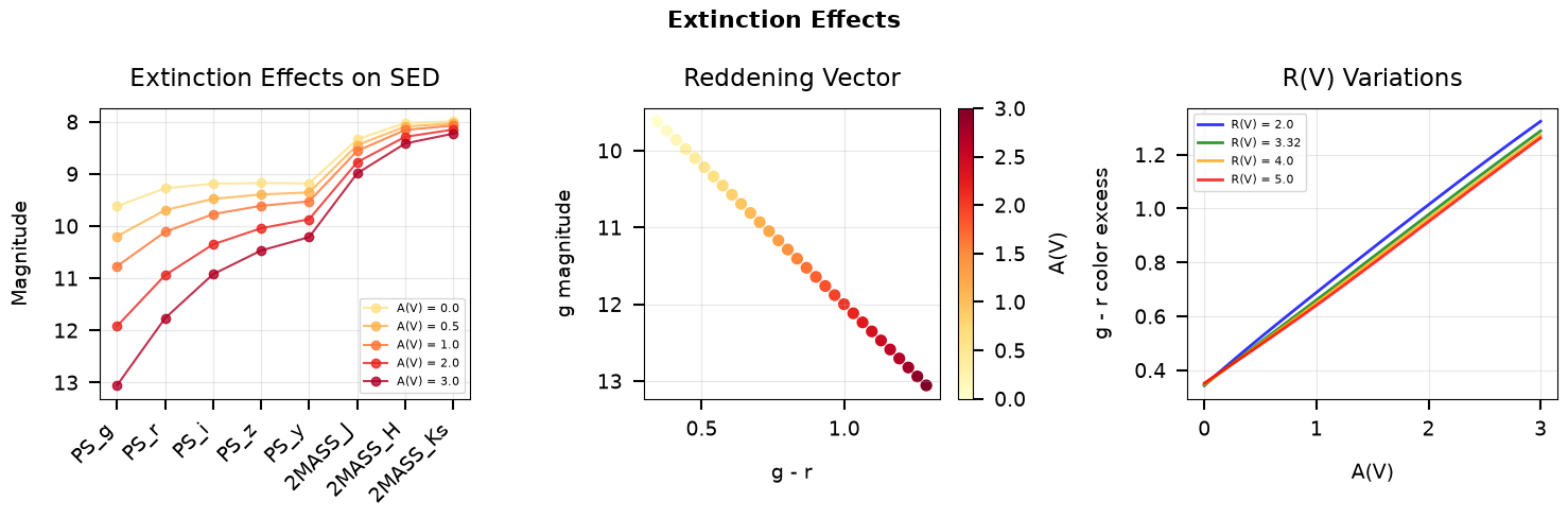
Extinction effects shown:
  - Extinction reddens and dims stars
  - R(V) controls extinction curve shape
Section 7: FastNN and FastNNPredictor#
FastNNPredictor (and its base class FastNN) provide a fast, lightweight alternative to StarEvolTrack for generating predicted magnitudes from stellar parameters.
How They Differ from StarEvolTrack#
StarEvolTrack takes evolutionary parameters (initial mass, EEP, metallicity) and internally resolves them to physical parameters (Teff, log g, luminosity, etc.) via the MIST evolutionary tracks, then feeds those into a neural network to get bolometric corrections and apparent magnitudes.
FastNNPredictor takes physical parameters directly (log Teff, log g, [Fe/H], log L, [alpha/Fe], Av, Rv, distance) and evaluates the neural network to produce apparent magnitudes, skipping the evolutionary track interpolation step entirely.
This makes FastNNPredictor useful when you already know the stellar parameters (e.g., from a catalog or a previous fit) and just need predicted photometry quickly. Since StarEvolTrack uses FastNNPredictor internally, the two should produce identical results when given the same physical parameters.
# Initialize FastNNPredictor with the same filters used earlier
try:
    from brutus.core import FastNNPredictor

    fastnn = FastNNPredictor(filters=filt, nnfile=str(nnfile), verbose=False)
    print(f"FastNNPredictor initialized with {fastnn.NFILT} filters: {', '.join(filt)}")

    # Predict magnitudes for a solar-like star at 1 kpc with mild extinction
    fastnn_mags = fastnn.sed(
        logt=3.76, logg=4.44, feh_surf=0.0, logl=0.0, afe=0.0,
        av=0.1, rv=3.3, dist=1000.0
    )

    print(f"\nFastNNPredictor magnitudes (logt=3.76, logg=4.44, feh=0.0, logl=0.0,")
    print(f"                            afe=0.0, av=0.1, rv=3.3, dist=1000 pc):\n")
    for f, m in zip(filt, fastnn_mags):
        print(f"  {f:10s}: {m:7.3f} mag")

    fastnn_available = True

except Exception as e:
    print(f"FastNNPredictor not available (data file missing?): {e}")
    print("Skipping FastNN examples. Run the download cell at the top to fetch data files.")
    fastnn_available = False
FastNNPredictor initialized with 8 filters: PS_g, PS_r, PS_i, PS_z, PS_y, 2MASS_J, 2MASS_H, 2MASS_Ks

FastNNPredictor magnitudes (logt=3.76, logg=4.44, feh=0.0, logl=0.0,
                            afe=0.0, av=0.1, rv=3.3, dist=1000 pc):

  PS_g      :  15.122 mag
  PS_r      :  14.711 mag
  PS_i      :  14.585 mag
  PS_z      :  14.546 mag
  PS_y      :  14.539 mag
  2MASS_J   :  13.669 mag
  2MASS_H   :  13.329 mag
  2MASS_Ks  :  13.290 mag
# Compare FastNNPredictor vs StarEvolTrack predictions
# StarEvolTrack resolves (mini, eep, feh) -> physical params -> magnitudes.
# We can extract the intermediate physical params and feed them directly
# to FastNNPredictor to verify the two paths give identical results.

if fastnn_available:
    # Use StarEvolTrack to get magnitudes AND the resolved physical parameters
    # for a 1 Msun ZAMS star at 1 kpc with mild extinction
    set_mags, set_params, _ = star.get_seds(
        mini=1.0, feh=0.0, eep=350, av=0.1, rv=3.3, dist=1000.0
    )

    # Now call FastNNPredictor with the same physical parameters
    fastnn_compare = fastnn.sed(
        logt=set_params['logt'],
        logg=set_params['logg'],
        feh_surf=set_params['feh_surf'],
        logl=set_params['logl'],
        afe=set_params['afe_surf'],
        av=0.1,
        rv=3.3,
        dist=1000.0,
    )

    # Print comparison table
    print("Comparison: StarEvolTrack vs FastNNPredictor")
    print("(Using identical physical params from a 1 Msun ZAMS star)\n")
    print(f"Resolved params: logt={set_params['logt']:.4f}, logg={set_params['logg']:.4f}, "
          f"feh_surf={set_params['feh_surf']:.4f}, logl={set_params['logl']:.4f}, "
          f"afe_surf={set_params['afe_surf']:.4f}\n")
    print(f"{'Filter':10s}  {'StarEvolTrack':>14s}  {'FastNNPredictor':>15s}  {'Difference':>10s}")
    print("-" * 55)
    for f, m_set, m_fnn in zip(filt, set_mags, fastnn_compare):
        diff = m_fnn - m_set
        print(f"{f:10s}  {m_set:14.4f}  {m_fnn:15.4f}  {diff:10.6f}")

    # Verify they match (should be identical since same NN is used)
    max_diff = np.max(np.abs(fastnn_compare - set_mags))
    print(f"\nMax absolute difference: {max_diff:.2e} mag")
    assert max_diff < 0.1, f"Predictions differ by more than 0.1 mag (max diff: {max_diff:.4f})"
    print("Assertion passed: all differences < 0.1 mag")
else:
    print("Skipping comparison (FastNNPredictor not available).")
Comparison: StarEvolTrack vs FastNNPredictor
(Using identical physical params from a 1 Msun ZAMS star)

Resolved params: logt=3.7662, logg=4.4321, feh_surf=-0.0143, logl=0.0256, afe_surf=0.0000

Filter       StarEvolTrack  FastNNPredictor  Difference
-------------------------------------------------------
PS_g               15.0376          15.0376    0.000000
PS_r               14.6473          14.6473    0.000000
PS_i               14.5309          14.5309    0.000000
PS_z               14.4992          14.4992    0.000000
PS_y               14.4958          14.4958    0.000000
2MASS_J            13.6341          13.6341    0.000000
2MASS_H            13.3069          13.3069    0.000000
2MASS_Ks           13.2696          13.2696    0.000000

Max absolute difference: 0.00e+00 mag
Assertion passed: all differences < 0.1 mag
Summary and Key Takeaways#
This tutorial has covered the fundamental components for modeling individual stars in brutus:
Key Classes#
EEPTracks: Provides stellar parameter predictions along evolutionary tracks
Interpolates MIST stellar evolution models
Returns physical parameters (Teff, log g, luminosity, age)
Covers full evolutionary phases from pre-MS to post-AGB
StarEvolTrack: Generates SEDs using neural networks
Fast bolometric corrections via neural networks
Supports any photometric filter system
Includes binary star modeling (SMF parameter)
Handles extinction (A(V), R(V)) and distance
FastNNPredictor: Lightweight SED prediction from physical parameters
Skips evolutionary track interpolation entirely
Takes physical parameters (Teff, log g, [Fe/H], L, Av, Rv) directly
Produces identical results to StarEvolTrack when given matching parameters
Useful when stellar parameters are already known
Physical Effects#
Metallicity: Affects temperature, color, and evolutionary timescales
Binaries: Create sequences above the main sequence
Extinction: Reddens and dims stellar light
Distance: Determines apparent magnitude via distance modulus
Next Steps#
Tutorial 2: Stellar Population Models (Isochrones and StellarPop)
Tutorial 3: Grid Generation and Performance Optimization
Tutorial 4: Galactic Priors and Population Synthesis
Tutorial 5: Fitting Individual Sources with BruteForce
print("Tutorial 1 Complete!")
print("="*60)
print("\nGenerated plots:")
for plot_file in sorted(plots_dir.glob('*.png')):
    print(f"  - {plot_file.name}")
Tutorial 1 Complete!
============================================================

Generated plots:
  - binary_modeling.png
  - extinction_distance.png
  - fastnn_residuals.png
  - metallicity_effects.png
  - sed_generation.png
  - stellar_evolution.png