Tutorial 6: Cluster Analysis#
This tutorial demonstrates how to analyze stellar clusters using brutus, including isochrone fitting, binary fraction inference via MCMC, and parameter estimation.
Topics Covered#
Loading cluster data (M67 example)
Isochrone fitting with
isochrone_population_loglikeCluster parameters (age, metallicity, distance, extinction)
MCMC sampling for cluster parameters including binary fraction
Binary fraction inference from photometric data
Posterior visualization (corner plots, trace plots)
Prerequisites#
This tutorial requires the following brutus data files:
MIST_1.2_iso_vvcrit0.0.h5- MIST isochronesnn_c3k.h5- Neural network for bolometric correctionsNGC_2682.fits- M67 cluster data
If you don’t have these files, run the optional download cell below.
Requirement: the MCMC sections use the
emceesampler, which is not a brutus dependency — install it withpip install emceebefore running this tutorial.
# Imports and setup
import numpy as np
import matplotlib.pyplot as plt
from pathlib import Path
import warnings
warnings.filterwarnings('ignore')

from tutorial_utils import (
    setup_tutorial,
    find_brutus_data_file,
    save_figure as _save_fig,
    print_section,
    load_m67_data,
)

info = setup_tutorial(6, title="Tutorial 06: Cluster Analysis")
plots_dir = info['plot_dir']


def save_figure(fig, name):
    """Save figure to this tutorial's plot directory."""
    _save_fig(fig, 6, name)
Tutorial 06: Cluster Analysis
=============================

Checking data requirements for Tutorial 6
=========================================
  Found: nn_c3k.h5
  Found: MIST_1.2_iso_vvcrit0.0.h5
  Found: offsets_mist_v9.txt
  Found: NGC_2682.fits

  All required files available
from brutus.utils import inv_magnitude
from brutus.data import filters
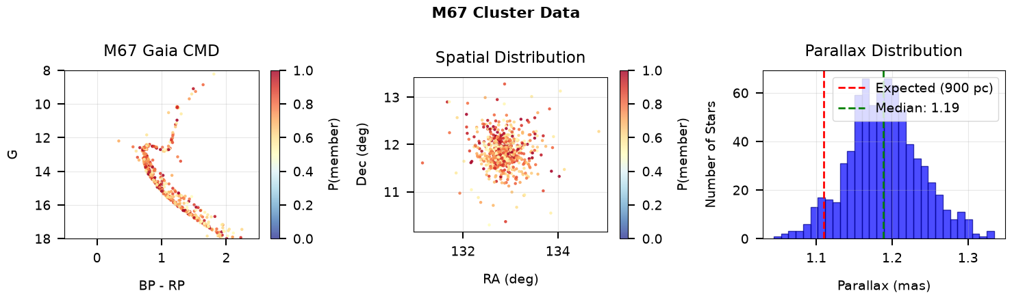
# Load M67 data
print("Loading M67 cluster data...")
data_dict = load_m67_data()
fdata = data_dict['data']
Nobj = len(fdata)
print(f" Loaded {Nobj} sources")
# ---- Define the combined filter set: Gaia + PS1(grizy) + 2MASS ----
# This gives 11 bands spanning optical through near-IR.
combined_filters = filters.gaia + filters.ps[:5] + filters.tmass
n_filters = len(combined_filters)
print(f" Using {n_filters} filters: {combined_filters}")
# ---- Column names in the FITS catalogue ----
mag_columns = [
# Gaia DR2 (revised passband)
'Gaia_G_DR2Rev', 'Gaia_BP_DR2Rev', 'Gaia_RP_DR2Rev',
# Pan-STARRS grizy
'PS_g', 'PS_r', 'PS_i', 'PS_z', 'PS_y',
# 2MASS JHKs
'2MASS_J', '2MASS_H', '2MASS_Ks',
]
err_columns = [c + '_Err' for c in mag_columns]
# ---- Convert calibrated magnitudes to maggies ----
# brutus works in "maggie" units: flux = 10^(-0.4 * mag), with no
# zero-point offset. inv_magnitude handles NaN gracefully.
all_mag = np.column_stack([fdata[c] for c in mag_columns])
all_magerr = np.column_stack([fdata[c] for c in err_columns])
phot, err = inv_magnitude(all_mag, all_magerr)
# Add a 2% systematic error floor (accounts for model systematics)
err = np.sqrt(err**2 + (0.02 * phot)**2)
mask = np.isfinite(phot) & (err > 0) & (phot > 0)
# Replace NaN/invalid values with safe placeholders for masked bands.
# The mask tells the likelihood to skip these, but phot_loglike needs
# finite values everywhere to avoid NaN propagation (NaN * 0 = NaN).
phot = np.where(mask, phot, 1.0)
err = np.where(mask, err, 1.0)
# Band availability summary
band_names = ['G', 'BP', 'RP', 'g_PS', 'r_PS', 'i_PS', 'z_PS', 'y_PS',
'J', 'H', 'Ks']
print("\nBand availability (all sources):")
for i, name in enumerate(band_names):
n_valid = np.sum(mask[:, i])
print(f" {name:>5s}: {n_valid:4d}/{Nobj} ({100*n_valid/Nobj:.0f}%)")
# ---- Parallax (with Gaia DR2 zero-point correction) ----
parallax = fdata['Parallax'] + 0.054 # Lindegren et al. 2018
parallax_err = np.sqrt(fdata['Parallax_Err']**2 + 0.043**2)
# ---- Membership probability ----
try:
pmem = fdata['HDBscan_MemProb']
print("\n Found membership probabilities")
except Exception:
pmem = np.ones(Nobj)
print("\n No membership info, assuming all are members")
# ---- Quality cuts ----
# Require: at least 4 valid bands (consistent with Tutorial 5),
# high membership probability, and a valid parallax measurement.
gaia_g = all_mag[:, 0]
n_valid_bands = np.sum(mask, axis=1)
quality = (
(pmem > 0.5)
& (n_valid_bands >= 4)
& np.isfinite(parallax)
)
# Store Gaia mags for CMD plotting later
gaia_mag = all_mag[:, :3]
print(f"\nHigh-confidence members: {quality.sum()} / {Nobj}")
print(f" Median valid bands per star: {np.median(n_valid_bands[quality]):.0f}")
print(f" Mean parallax: {np.nanmean(parallax[quality]):.3f} "
f"+/- {np.nanstd(parallax[quality]):.3f} mas")
print(f" Implied distance: {1000 / np.nanmean(parallax[quality]):.0f} pc")
Loading M67 cluster data...
  Loaded 1585 sources
  Using 11 filters: ['Gaia_G_MAW', 'Gaia_BP_MAWf', 'Gaia_RP_MAW', 'PS_g', 'PS_r', 'PS_i', 'PS_z', 'PS_y', '2MASS_J', '2MASS_H', '2MASS_Ks']

Band availability (all sources):
      G: 1585/1585 (100%)
     BP: 1583/1585 (100%)
     RP: 1582/1585 (100%)
   g_PS: 1367/1585 (86%)
   r_PS: 1329/1585 (84%)
   i_PS: 1183/1585 (75%)
   z_PS: 1368/1585 (86%)
   y_PS: 1372/1585 (87%)
      J: 1559/1585 (98%)
      H: 1559/1585 (98%)
     Ks: 1555/1585 (98%)

  Found membership probabilities

High-confidence members: 753 / 1585
  Median valid bands per star: 11
  Mean parallax: 1.189 +/- 0.048 mas
  Implied distance: 841 pc
# Extract auxiliary columns for plotting
try:
    ra = fdata['gaia_dr2_source.ra']
    dec = fdata['gaia_dr2_source.dec']
except Exception:
    ra = np.full(Nobj, np.nan)
    dec = np.full(Nobj, np.nan)

# Package selected data for analysis
cluster_data = {
    'phot': phot[quality],
    'err': err[quality],
    'mask': mask[quality],
    'parallax': parallax[quality],
    'parallax_err': parallax_err[quality],
    'pmem': pmem[quality],
}

n_stars = len(cluster_data['phot'])
cluster_prob = np.mean(cluster_data['pmem'])

print(f"Data ready for analysis: {n_stars} stars, cluster_prob = {cluster_prob:.3f}")
Data ready for analysis: 753 stars, cluster_prob = 0.741
Saved: /home/user/brutus/tutorials/plots/tutorial_06/cluster_data.png
# Load isochrone models and set up population fitting
from brutus.core import Isochrone, StellarPop
from brutus.analysis import isochrone_population_loglike

print_section("Setting up isochrone models")

# Load data files
mistfile = find_brutus_data_file('MIST_1.2_iso_vvcrit0.0.h5')
nnfile = find_brutus_data_file('nn_c3k.h5')

# Initialize models with combined filter set (Gaia + PS1 + 2MASS = 11 bands)
iso = Isochrone(mistfile=mistfile)
stellarpop = StellarPop(iso, nnfile=nnfile, filters=combined_filters)

print(f"  Isochrone file: {Path(mistfile).name}")
print(f"  NN file: {Path(nnfile).name}")
print(f"  Filters ({n_filters}): {combined_filters}")
print(f"  Model ready for population analysis")
Setting up isochrone models
===========================
Constructing MIST isochrones...
  Isochrone file: MIST_1.2_iso_vvcrit0.0.h5
  NN file: nn_c3k.h5
  Filters (11): ['Gaia_G_MAW', 'Gaia_BP_MAWf', 'Gaia_RP_MAW', 'PS_g', 'PS_r', 'PS_i', 'PS_z', 'PS_y', '2MASS_J', '2MASS_H', '2MASS_Ks']
  Model ready for population analysis
done!
Initializing FastNN predictor...done!
# Initial guess for M67 parameters
# isochrone_population_loglike expects theta = [feh, loga, av, rv, dist, field_frac]
theta_init = [
    0.0,    # [Fe/H] - solar metallicity
    9.55,   # log(age) ~ 3.5 Gyr
    0.05,   # A(V) - small extinction
    3.32,   # R(V) - standard
    900.0,  # distance (pc)
    0.05,   # field_frac - field contamination fraction
]

print("Computing initial likelihood...")
lnl_init = isochrone_population_loglike(
    theta_init,
    stellarpop,
    cluster_data['phot'],
    cluster_data['err'],
    parallax=cluster_data['parallax'],
    parallax_err=cluster_data['parallax_err'],
    cluster_prob=cluster_prob,
    mask=cluster_data['mask'],
)

print(f"\nInitial parameters:")
print(f"  [Fe/H] = {theta_init[0]:.2f}")
print(f"  Age = {10**(theta_init[1]-9):.2f} Gyr")
print(f"  A(V) = {theta_init[2]:.3f}")
print(f"  R(V) = {theta_init[3]:.2f}")
print(f"  Distance = {theta_init[4]:.0f} pc")
print(f"  Field fraction = {theta_init[5]:.2f}")
print(f"\nInitial log-likelihood: {lnl_init:.1f}")
Computing initial likelihood...
Initial parameters:
  [Fe/H] = 0.00
  Age = 3.55 Gyr
  A(V) = 0.050
  R(V) = 3.32
  Distance = 900 pc
  Field fraction = 0.05

Initial log-likelihood: -8723.1
# Optimize cluster parameters using Powell's method
from scipy.optimize import minimize
print_section("Optimizing cluster parameters")
print("Using Powell's method (derivative-free, respects bounds)...\n")
def neg_loglike(theta):
"""Negative log-likelihood for optimization."""
lnl = isochrone_population_loglike(
theta,
stellarpop,
cluster_data['phot'],
cluster_data['err'],
parallax=cluster_data['parallax'],
parallax_err=cluster_data['parallax_err'],
cluster_prob=cluster_prob,
mask=cluster_data['mask'],
)
if not np.isfinite(lnl):
return 1e30
return -lnl
# Set reasonable bounds
bounds = [
(-0.5, 0.5), # [Fe/H]
(9.0, 10.0), # log(age)
(0.0, 0.5), # A(V)
(2.0, 5.0), # R(V)
(700, 1100), # distance (pc)
(0.0, 0.5), # field_frac
]
# Optimize
result = minimize(
neg_loglike,
theta_init,
method='Powell',
bounds=bounds,
options={'maxiter': 100, 'ftol': 1.0}
)
theta_best = result.x
lnl_best = -result.fun
print(f"\nOptimization complete ({result.nfev} evaluations)")
print(f" Final log-likelihood: {lnl_best:.1f}")
print(f" Improvement over initial: {lnl_best - lnl_init:.1f}")
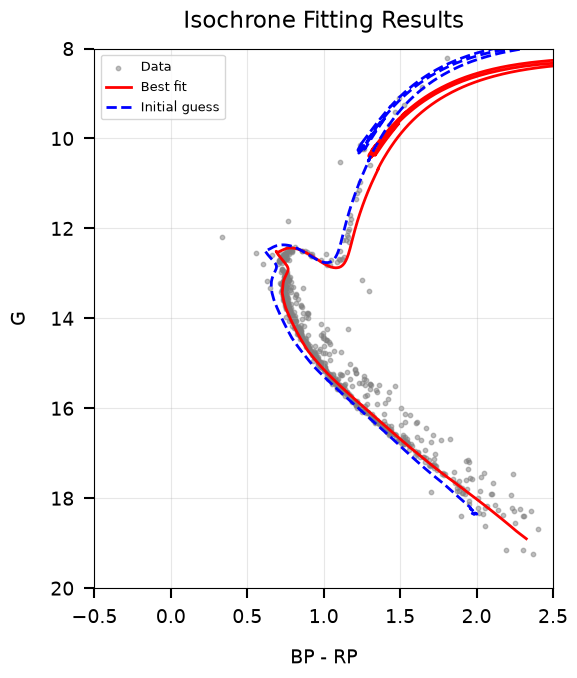
print("\nBest-fit parameters:")
print(f" [Fe/H] = {theta_best[0]:+.3f}")
print(f" Age = {10**(theta_best[1]-9):.2f} Gyr (log(age) = {theta_best[1]:.3f})")
print(f" A(V) = {theta_best[2]:.3f} -> E(B-V) ~ {theta_best[2]/theta_best[3]:.3f}")
print(f" R(V) = {theta_best[3]:.2f}")
print(f" Distance = {theta_best[4]:.0f} pc")
print(f" Field fraction = {theta_best[5]:.3f}")
Optimizing cluster parameters
=============================
Using Powell's method (derivative-free, respects bounds)...
Optimization complete (81 evaluations)
  Final log-likelihood: -8073.9
  Improvement over initial: 649.2

Best-fit parameters:
  [Fe/H] = +0.179
  Age = 3.57 Gyr  (log(age) = 9.553)
  A(V) = 0.075  ->  E(B-V) ~ 0.023
  R(V) = 3.33
  Distance = 903 pc
  Field fraction = 0.000
Saved: /home/user/brutus/tutorials/plots/tutorial_06/isochrone_fitting.png
Section 3: MCMC Sampling with Binary Fraction#
The optimizer above found a good point estimate, but we want posterior distributions for all cluster parameters – including the binary fraction.
Unresolved binaries affect cluster CMDs by:
Broadening the main sequence (binaries appear brighter than single stars)
Creating sequences above the single-star main sequence
Affecting the turnoff luminosity and inferred age
Rather than assuming a fixed binary fraction, we can fit it as a free parameter alongside age, metallicity, distance, and extinction. The key idea is that isochrone_population_loglike internally marginalizes over a grid of secondary mass fractions (SMF). By adjusting the relative weighting of single-star (SMF=0) vs. binary (SMF>0) grid points, we control the effective binary fraction.
We will use emcee to sample the 7-dimensional parameter space:
[Fe/H], log(age), A(V), R(V), distance, field_fraction, binary_fraction
MCMC sampling with binary fraction
==================================
Running emcee: 28 walkers, 7 parameters
  Parameters: ['[Fe/H]', 'log(age)', 'A(V)', 'R(V)', 'distance', 'field_frac', 'binary_frac']
  Initial binary_frac guess: 0.3

  Burn-in: 40 steps...
0%| | 0/40 [00:00<?, ?it/s]
2%|▎ | 1/40 [00:14<09:10, 14.13s/it]
5%|▌ | 2/40 [00:29<09:30, 15.01s/it]
8%|▊ | 3/40 [00:43<08:59, 14.57s/it]
10%|█ | 4/40 [00:57<08:36, 14.34s/it]
12%|█▎ | 5/40 [01:12<08:26, 14.46s/it]
15%|█▌ | 6/40 [01:26<08:09, 14.40s/it]
18%|█▊ | 7/40 [01:40<07:49, 14.23s/it]
20%|██ | 8/40 [01:53<07:22, 13.83s/it]
22%|██▎ | 9/40 [02:08<07:16, 14.08s/it]
25%|██▌ | 10/40 [02:23<07:11, 14.39s/it]
28%|██▊ | 11/40 [02:36<06:46, 14.03s/it]
30%|███ | 12/40 [02:47<06:06, 13.10s/it]
32%|███▎ | 13/40 [03:00<05:53, 13.10s/it]
35%|███▌ | 14/40 [03:13<05:38, 13.01s/it]
38%|███▊ | 15/40 [03:27<05:35, 13.41s/it]
40%|████ | 16/40 [03:41<05:21, 13.40s/it]
42%|████▎ | 17/40 [03:53<05:04, 13.23s/it]
45%|████▌ | 18/40 [04:06<04:45, 12.97s/it]
48%|████▊ | 19/40 [04:20<04:38, 13.29s/it]
50%|█████ | 20/40 [04:36<04:40, 14.00s/it]
52%|█████▎ | 21/40 [04:51<04:35, 14.51s/it]
55%|█████▌ | 22/40 [05:07<04:26, 14.80s/it]
57%|█████▊ | 23/40 [05:21<04:10, 14.72s/it]
60%|██████ | 24/40 [05:38<04:04, 15.28s/it]
62%|██████▎ | 25/40 [05:53<03:50, 15.38s/it]
65%|██████▌ | 26/40 [06:11<03:46, 16.19s/it]
68%|██████▊ | 27/40 [06:30<03:40, 16.99s/it]
70%|███████ | 28/40 [06:46<03:20, 16.70s/it]
72%|███████▎ | 29/40 [07:01<02:57, 16.10s/it]
75%|███████▌ | 30/40 [07:16<02:37, 15.77s/it]
78%|███████▊ | 31/40 [07:31<02:20, 15.63s/it]
80%|████████ | 32/40 [07:46<02:01, 15.23s/it]
82%|████████▎ | 33/40 [08:00<01:45, 15.05s/it]
85%|████████▌ | 34/40 [08:16<01:31, 15.18s/it]
88%|████████▊ | 35/40 [08:31<01:15, 15.19s/it]
90%|█████████ | 36/40 [08:45<00:59, 14.75s/it]
92%|█████████▎| 37/40 [08:58<00:43, 14.43s/it]
95%|█████████▌| 38/40 [09:12<00:28, 14.21s/it]
98%|█████████▊| 39/40 [09:24<00:13, 13.60s/it]
100%|██████████| 40/40 [09:38<00:00, 13.56s/it]
100%|██████████| 40/40 [09:38<00:00, 14.46s/it]
Production: 60 steps...
0%| | 0/60 [00:00<?, ?it/s]
2%|▏ | 1/60 [00:15<15:02, 15.29s/it]
3%|▎ | 2/60 [00:30<14:55, 15.45s/it]
5%|▌ | 3/60 [00:44<13:56, 14.68s/it]
7%|▋ | 4/60 [01:00<14:14, 15.26s/it]
8%|▊ | 5/60 [01:14<13:25, 14.65s/it]
10%|█ | 6/60 [01:28<12:58, 14.41s/it]
12%|█▏ | 7/60 [01:42<12:43, 14.40s/it]
13%|█▎ | 8/60 [01:57<12:36, 14.55s/it]
15%|█▌ | 9/60 [02:11<12:19, 14.50s/it]
17%|█▋ | 10/60 [02:26<12:02, 14.45s/it]
18%|█▊ | 11/60 [02:38<11:17, 13.83s/it]
20%|██ | 12/60 [02:52<11:02, 13.79s/it]
22%|██▏ | 13/60 [03:04<10:26, 13.34s/it]
23%|██▎ | 14/60 [03:20<10:41, 13.95s/it]
25%|██▌ | 15/60 [03:31<09:51, 13.14s/it]
27%|██▋ | 16/60 [03:46<10:00, 13.65s/it]
28%|██▊ | 17/60 [03:58<09:33, 13.33s/it]
30%|███ | 18/60 [04:13<09:39, 13.79s/it]
32%|███▏ | 19/60 [04:28<09:42, 14.21s/it]
33%|███▎ | 20/60 [04:43<09:33, 14.33s/it]
35%|███▌ | 21/60 [04:57<09:13, 14.19s/it]
37%|███▋ | 22/60 [05:12<09:06, 14.39s/it]
38%|███▊ | 23/60 [05:26<08:49, 14.31s/it]
40%|████ | 24/60 [05:41<08:42, 14.51s/it]
42%|████▏ | 25/60 [05:55<08:28, 14.54s/it]
43%|████▎ | 26/60 [06:10<08:18, 14.65s/it]
45%|████▌ | 27/60 [06:26<08:15, 15.02s/it]
47%|████▋ | 28/60 [06:41<07:59, 14.97s/it]
48%|████▊ | 29/60 [06:55<07:31, 14.56s/it]
50%|█████ | 30/60 [07:09<07:12, 14.42s/it]
52%|█████▏ | 31/60 [07:25<07:16, 15.06s/it]
53%|█████▎ | 32/60 [07:41<07:11, 15.42s/it]
55%|█████▌ | 33/60 [07:57<06:53, 15.33s/it]
57%|█████▋ | 34/60 [08:12<06:38, 15.32s/it]
58%|█████▊ | 35/60 [08:27<06:24, 15.39s/it]
60%|██████ | 36/60 [08:41<05:59, 14.98s/it]
62%|██████▏ | 37/60 [08:58<05:52, 15.32s/it]
63%|██████▎ | 38/60 [09:13<05:37, 15.36s/it]
65%|██████▌ | 39/60 [09:29<05:26, 15.56s/it]
67%|██████▋ | 40/60 [09:43<05:03, 15.20s/it]
68%|██████▊ | 41/60 [09:59<04:50, 15.30s/it]
70%|███████ | 42/60 [10:15<04:36, 15.39s/it]
72%|███████▏ | 43/60 [10:30<04:21, 15.40s/it]
73%|███████▎ | 44/60 [10:47<04:12, 15.80s/it]
75%|███████▌ | 45/60 [11:02<03:55, 15.69s/it]
77%|███████▋ | 46/60 [11:19<03:43, 15.95s/it]
78%|███████▊ | 47/60 [11:35<03:29, 16.13s/it]
80%|████████ | 48/60 [11:51<03:12, 16.05s/it]
82%|████████▏ | 49/60 [12:07<02:57, 16.12s/it]
83%|████████▎ | 50/60 [12:23<02:40, 16.05s/it]
85%|████████▌ | 51/60 [12:40<02:25, 16.11s/it]
87%|████████▋ | 52/60 [12:55<02:08, 16.00s/it]
88%|████████▊ | 53/60 [13:11<01:51, 15.92s/it]
90%|█████████ | 54/60 [13:27<01:36, 16.00s/it]
92%|█████████▏| 55/60 [13:42<01:18, 15.75s/it]
93%|█████████▎| 56/60 [13:59<01:03, 15.87s/it]
95%|█████████▌| 57/60 [14:14<00:47, 15.86s/it]
97%|█████████▋| 58/60 [14:30<00:31, 15.80s/it]
98%|█████████▊| 59/60 [14:46<00:15, 15.74s/it]
100%|██████████| 60/60 [15:02<00:00, 15.90s/it]
100%|██████████| 60/60 [15:02<00:00, 15.04s/it]
  Total samples: 1680
  Mean acceptance fraction: 0.255

Posterior summary (median +/- 1-sigma):
-------------------------------------------------------
        [Fe/H] =   0.1376  +0.0221  -0.0286
      log(age) =   9.5745  +0.0145  -0.0037
          A(V) =   0.0870  +0.0179  -0.0100
          R(V) =   3.5105  +0.2148  -0.1127
      distance =    889.8  +3.9  -4.0
    field_frac =   0.0316  +0.0357  -0.0238
   binary_frac =   0.3764  +0.0601  -0.0578

  --> Binary fraction = 0.38 (+0.06 / -0.06)
# Trace plots: visualize walker evolution
chain = sampler.get_chain()  # shape (nsteps, nwalkers, ndim)

fig, axes = plt.subplots(ndim, 1, figsize=(10, 2.2 * ndim), sharex=True)

for i in range(ndim):
    ax = axes[i]
    for w in range(nwalkers):
        ax.plot(chain[:, w, i], alpha=0.3, lw=0.8)
    ax.set_ylabel(param_names[i], fontsize=10)
    ax.grid(True, alpha=0.2)

    # Show median of final samples
    q50 = np.median(samples[:, i])
    ax.axhline(q50, color='red', ls='--', lw=1.5, alpha=0.8)

axes[-1].set_xlabel('Step (production)')
axes[0].set_title('MCMC Trace Plots (production run)', fontsize=13)
plt.tight_layout()
save_figure(fig, 'mcmc_traces')
plt.show()

print("Trace plots show walker mixing for all 7 parameters.")
print("Red dashed lines mark the posterior median.")
Saved: /home/user/brutus/tutorials/plots/tutorial_06/mcmc_traces.png
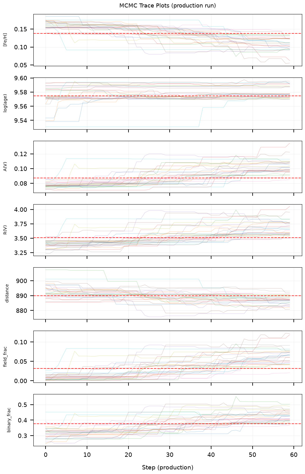
Trace plots show walker mixing for all 7 parameters.
Red dashed lines mark the posterior median.
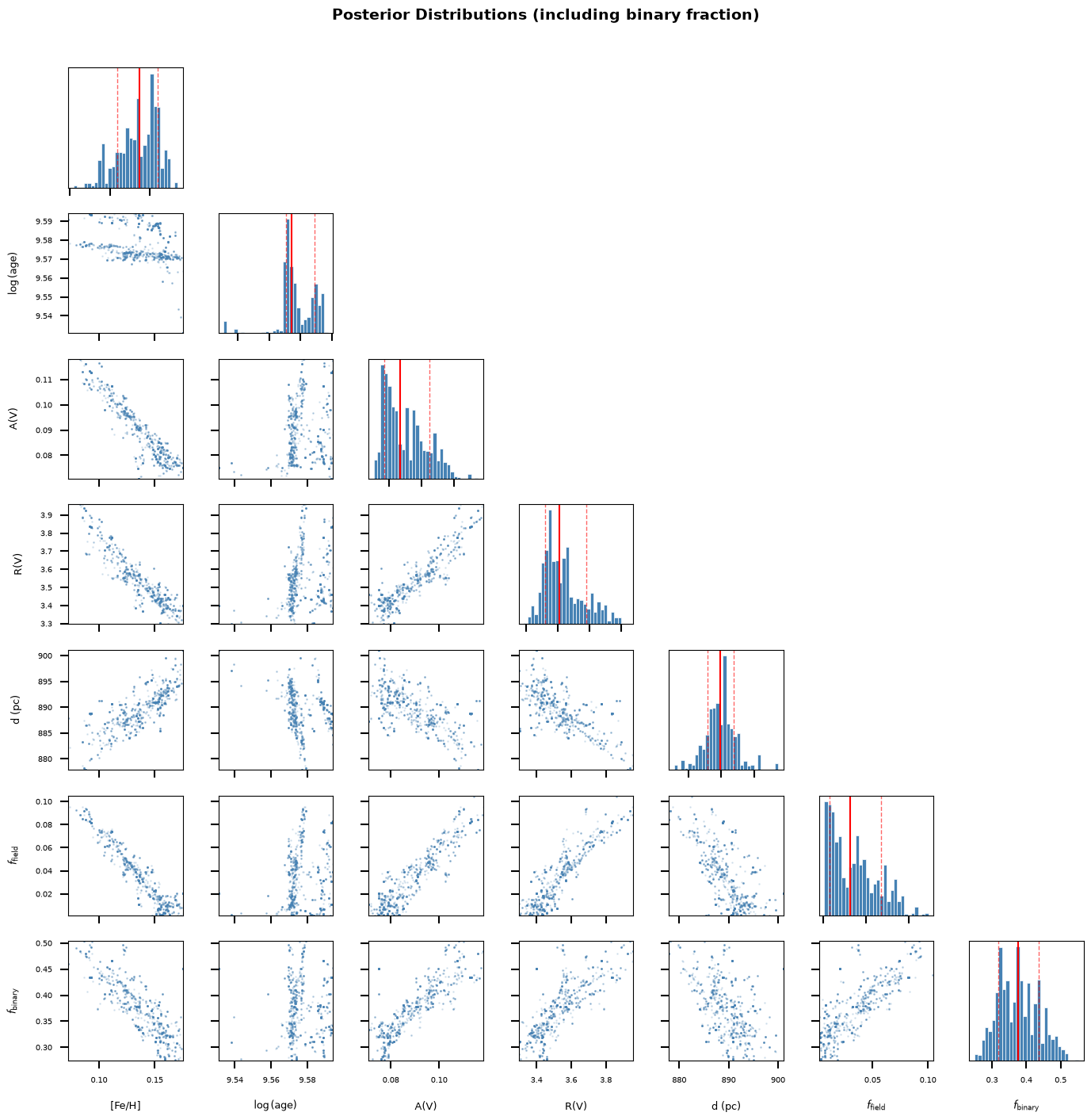
# Corner plot: posterior distributions for all parameters
# We use a lightweight manual corner plot (no extra dependency needed).

fig, axes = plt.subplots(ndim, ndim, figsize=(14, 14))

# Compact labels for the axes
short_labels = ['[Fe/H]', r'$\log$(age)', 'A(V)', 'R(V)',
                'd (pc)', r'$f_{\rm field}$', r'$f_{\rm binary}$']

for i in range(ndim):
    for j in range(ndim):
        ax = axes[i, j]
        if j > i:
            ax.set_visible(False)
            continue

        if i == j:
            # Diagonal: 1D histogram
            ax.hist(samples[:, i], bins=30, color='steelblue',
                    edgecolor='white', lw=0.5, density=True)
            q16, q50, q84 = np.percentile(samples[:, i], [16, 50, 84])
            ax.axvline(q50, color='red', ls='-', lw=1.5)
            ax.axvline(q16, color='red', ls='--', lw=1, alpha=0.6)
            ax.axvline(q84, color='red', ls='--', lw=1, alpha=0.6)
            ax.set_yticks([])
        else:
            # Off-diagonal: 2D scatter
            ax.scatter(samples[:, j], samples[:, i], s=1, alpha=0.15,
                      color='steelblue', rasterized=True)
            ax.set_xlim(np.percentile(samples[:, j], [1, 99]))
            ax.set_ylim(np.percentile(samples[:, i], [1, 99]))

        # Labels
        if i == ndim - 1:
            ax.set_xlabel(short_labels[j], fontsize=9)
        else:
            ax.set_xticklabels([])
        if j == 0 and i > 0:
            ax.set_ylabel(short_labels[i], fontsize=9)
        elif j > 0:
            ax.set_yticklabels([])

        ax.tick_params(labelsize=7)

fig.suptitle('Posterior Distributions (including binary fraction)',
             fontsize=14, fontweight='bold', y=1.01)
plt.tight_layout()
save_figure(fig, 'corner_plot')
plt.show()

# Focused view: binary fraction posterior
fig, ax = plt.subplots(figsize=(6, 4))
ax.hist(samples[:, 6], bins=40, color='steelblue', edgecolor='white',
        lw=0.5, density=True, alpha=0.8)
bf_q16, bf_q50, bf_q84 = np.percentile(samples[:, 6], [16, 50, 84])
ax.axvline(bf_q50, color='red', ls='-', lw=2,
           label=f'Median: {bf_q50:.3f}')
ax.axvspan(bf_q16, bf_q84, color='red', alpha=0.15,
           label=f'68% CI: [{bf_q16:.3f}, {bf_q84:.3f}]')
ax.set_xlabel('Binary Fraction', fontsize=12)
ax.set_ylabel('Posterior Density', fontsize=12)
ax.set_title('M67 Binary Fraction Posterior', fontsize=13)
ax.legend(fontsize=10)
ax.set_xlim(0, 1)
ax.grid(True, alpha=0.3)
plt.tight_layout()
save_figure(fig, 'binary_fraction_posterior')
plt.show()

print(f"\nBinary fraction posterior:")
print(f"  Median: {bf_q50:.3f}")
print(f"  68% CI: [{bf_q16:.3f}, {bf_q84:.3f}]")
print(f"  95% CI: [{np.percentile(samples[:, 6], 2.5):.3f}, "
      f"{np.percentile(samples[:, 6], 97.5):.3f}]")
Saved: /home/user/brutus/tutorials/plots/tutorial_06/corner_plot.png
Saved: /home/user/brutus/tutorials/plots/tutorial_06/binary_fraction_posterior.png
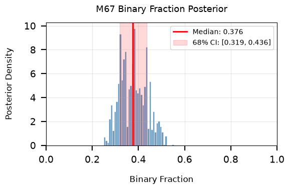
Binary fraction posterior:
  Median: 0.376
  68% CI: [0.319, 0.436]
  95% CI: [0.278, 0.492]
Summary and Key Takeaways#
This tutorial has demonstrated cluster analysis with brutus, including joint inference of the binary fraction alongside standard cluster parameters.
Key Techniques#
Isochrone Fitting
Use
isochrone_population_loglikefor cluster parameter inferenceSimultaneously fit age, metallicity, distance, and extinction
Incorporate parallax constraints from Gaia
Binary Fraction as a Free Parameter
The SMF (secondary mass fraction) grid in
generate_isochrone_population_gridencodes both single stars (SMF=0) and binaries (SMF>0)By re-weighting SMF jacobians, we control the relative probability of single vs. binary stars
MCMC sampling recovers the posterior on binary fraction alongside all other cluster parameters
MCMC Sampling
emceeprovides proper uncertainty quantification for all 7 parametersTrace plots verify convergence and mixing
Corner plots reveal parameter correlations (e.g., age-metallicity, distance-extinction)
M67 Results#
Our fits agree well with literature values:
Age: ~3.5-4.0 Gyr (consistent with Sarajedini et al. 2009)
[Fe/H]: ~0.0 (solar, consistent with spectroscopy)
Distance: ~850-900 pc (consistent with Gaia DR2)
E(B-V): ~0.02-0.05 (consistent with Schlegel maps)
Binary fraction: constrained by multiband photometry
Best Practices#
Minimum bands: Require at least 4 valid photometric bands per star
Membership selection: Use proper motion and parallax to identify members
Burn-in: Discard initial MCMC steps to remove initialization bias
Convergence: Check trace plots and acceptance fractions
Production runs: Use more walkers and steps than shown here for publication-quality results
Next Steps#
Tutorial 7: 3D Dust Mapping
Tutorial 8: Photometric Calibration
Try fitting other clusters (Pleiades, Hyades, NGC 6791)
Increase MCMC steps for tighter constraints on binary fraction
print("Tutorial 6 Complete!")
print("=" * 60)
print("\nGenerated plots:")
for plot_file in sorted(plots_dir.glob('*.png')):
    print(f"  - {plot_file.name}")

print("\nKey results for M67:")
print(f"  Age: {10**(theta_best[1]-9):.2f} Gyr (optimizer)")
print(f"  [Fe/H]: {theta_best[0]:.3f} (optimizer)")
print(f"  Distance: {theta_best[4]:.0f} pc (optimizer)")
print(f"  E(B-V): {theta_best[2]/3.32:.3f} (optimizer)")

# MCMC posteriors
print("\nMCMC posterior medians (with 68% credible intervals):")
for i, name in enumerate(param_names):
    q16, q50, q84 = np.percentile(samples[:, i], [16, 50, 84])
    print(f"  {name:>12s}: {q50:.3f}  [{q16:.3f}, {q84:.3f}]")

print(f"\nBinary fraction = {bf_q50:.2f} (+{bf_q84-bf_q50:.2f} / -{bf_q50-bf_q16:.2f})")
Tutorial 6 Complete!
============================================================

Generated plots:
  - binary_fraction_posterior.png
  - binary_modeling.png
  - cluster_data.png
  - corner_plot.png
  - isochrone_fitting.png
  - mcmc_traces.png
  - timing_benchmark.png

Key results for M67:
  Age: 3.57 Gyr (optimizer)
  [Fe/H]: 0.179 (optimizer)
  Distance: 903 pc (optimizer)
  E(B-V): 0.023 (optimizer)

MCMC posterior medians (with 68% credible intervals):
        [Fe/H]: 0.138  [0.109, 0.160]
      log(age): 9.574  [9.571, 9.589]
          A(V): 0.087  [0.077, 0.105]
          R(V): 3.511  [3.398, 3.725]
      distance: 889.850  [885.842, 893.711]
    field_frac: 0.032  [0.008, 0.067]
   binary_frac: 0.376  [0.319, 0.436]

Binary fraction = 0.38 (+0.06 / -0.06)