Tutorial 2: Stellar Population Models

This tutorial explores stellar population modeling using Isochrone and StellarPop classes.

Topics Covered

1. Isochrone class for coeval stellar populations

2. StellarPop for population synthesis

3. Age and metallicity sequences

4. IMF sampling and mass functions

5. Synthetic cluster generation

Prerequisites

This tutorial requires the following brutus data files:

• MIST_1.2_iso_vvcrit0.0.h5 - MIST isochrones

• nn_c3k.h5 - Neural network for bolometric corrections

If you don’t have these files, run the optional download cell below.

# Optional: Download required data files (only needed if not already cached)
# This tutorial requires MIST isochrones and the C3K neural network.
# Uncomment the lines below to download them (~250 MB total).

# from brutus.data import fetch_isos, fetch_nns
# fetch_isos()       # ~200 MB -- MIST isochrones
# fetch_nns()        # ~50 MB  -- Neural network for bolometric corrections

# Imports and setup
import numpy as np
import matplotlib.pyplot as plt
import warnings
warnings.filterwarnings('ignore')

from tutorial_utils import (
    setup_tutorial,
    find_brutus_data_file,
    save_figure as _save_fig,
    print_section,
)

info = setup_tutorial(2, title="Tutorial 02: Stellar Population Models")
plots_dir = info['plot_dir']


def save_figure(fig, name):
    """Save figure to this tutorial's plot directory."""
    _save_fig(fig, 2, name)

Tutorial 02: Stellar Population Models
======================================

Checking data requirements for Tutorial 2
=========================================
  Found: nn_c3k.h5
  Found: MIST_1.2_iso_vvcrit0.0.h5

  All required files available

Section 1: Understanding Isochrones

Isochrones model populations of stars born at the same time with the same composition. They are fundamental for understanding star clusters and stellar populations in galaxies.

Key Concepts

• Isochrone: A line in the HR diagram connecting stars of the same age and composition but different masses

• Coeval population: All stars formed at the same time (e.g., star clusters)

• EEP grid: Equivalent Evolutionary Points provide consistent sampling across different masses

from brutus.core import Isochrone
from brutus.data import filters

# Initialize Isochrone
print("Loading MIST isochrones...")
mistfile = find_brutus_data_file('MIST_1.2_iso_vvcrit0.0.h5')

# Note: Isochrone doesn't take nnfile or filters as arguments
iso = Isochrone(mistfile=mistfile, verbose=False)

print(f"Loaded isochrones")
print(f"  Age range: {iso.loga_grid.min():.1f} - {iso.loga_grid.max():.1f} log(years)")
print(f"  Metallicity range: {iso.feh_grid.min():.2f} - {iso.feh_grid.max():.2f}")
print(f"  Available predictions: {iso.predictions}")

Loading MIST isochrones...

Loaded isochrones
  Age range: 5.0 - 10.3 log(years)
  Metallicity range: -4.00 - 0.50
  Available predictions: ['mini', 'mass', 'logl', 'logt', 'logr', 'logg', 'feh_surf', 'afe_surf']

# Generate a sample isochrone
print("\nGenerating 1 Gyr solar metallicity isochrone...")

# Set EEP grid (covers full evolution)
eep_grid = np.linspace(202, 808, 2000)

# Generate isochrone parameters
params_arr = iso.get_predictions(feh=0.0, afe=0.0, loga=9.0, eep=eep_grid)

# Convert to structured array for easier access
params = {}
for i, label in enumerate(iso.predictions):
    params[label] = params_arr[:, i]

# Find valid points (where mass exists)
valid = np.isfinite(params['mini'])
print(f"  Valid EEP points: {valid.sum()}/{len(eep_grid)}")
print(f"  Mass range: {params['mini'][valid].min():.2f} - {params['mini'][valid].max():.2f} M☉")

# Show some example stellar parameters
print("\nExample stellar parameters along isochrone:")
for i in [100, 500, 900, 1300]:
    if i < len(params['mini']) and np.isfinite(params['mini'][i]):
        print(f"  Star {i}: M={params['mini'][i]:.2f} M☉, "
              f"Teff={10**params['logt'][i]:.0f} K, "
              f"L={10**params['logl'][i]:.2f} L☉")

Generating 1 Gyr solar metallicity isochrone...
  Valid EEP points: 2000/2000
  Mass range: 0.14 - 2.29 M☉

Example stellar parameters along isochrone:
  Star 100: M=0.35 M☉, Teff=3312 K, L=0.02 L☉
  Star 500: M=1.77 M☉, Teff=7704 K, L=14.07 L☉
  Star 900: M=2.05 M☉, Teff=6323 K, L=37.01 L☉
  Star 1300: M=2.07 M☉, Teff=4397 K, L=169.89 L☉

Section 2: StellarPop for Population Synthesis

StellarPop generates synthetic stellar populations by sampling from an IMF and computing population-level photometry including binaries.

Key Features

• Combines Isochrone predictions with neural network photometry

• Handles binary star populations

• Applies extinction and distance effects

• Generates realistic synthetic clusters

from brutus.core import StellarPop

# Initialize StellarPop with photometric filters
nnfile = find_brutus_data_file('nn_c3k.h5')
filt = filters.gaia + filters.ps[:3]

print(f"Using filters: {', '.join(filt)}")

# Create StellarPop instance
pop = StellarPop(isochrone=iso, filters=filt, nnfile=nnfile, verbose=False)

print("StellarPop initialized")

Using filters: Gaia_G_MAW, Gaia_BP_MAWf, Gaia_RP_MAW, PS_g, PS_r, PS_i
StellarPop initialized

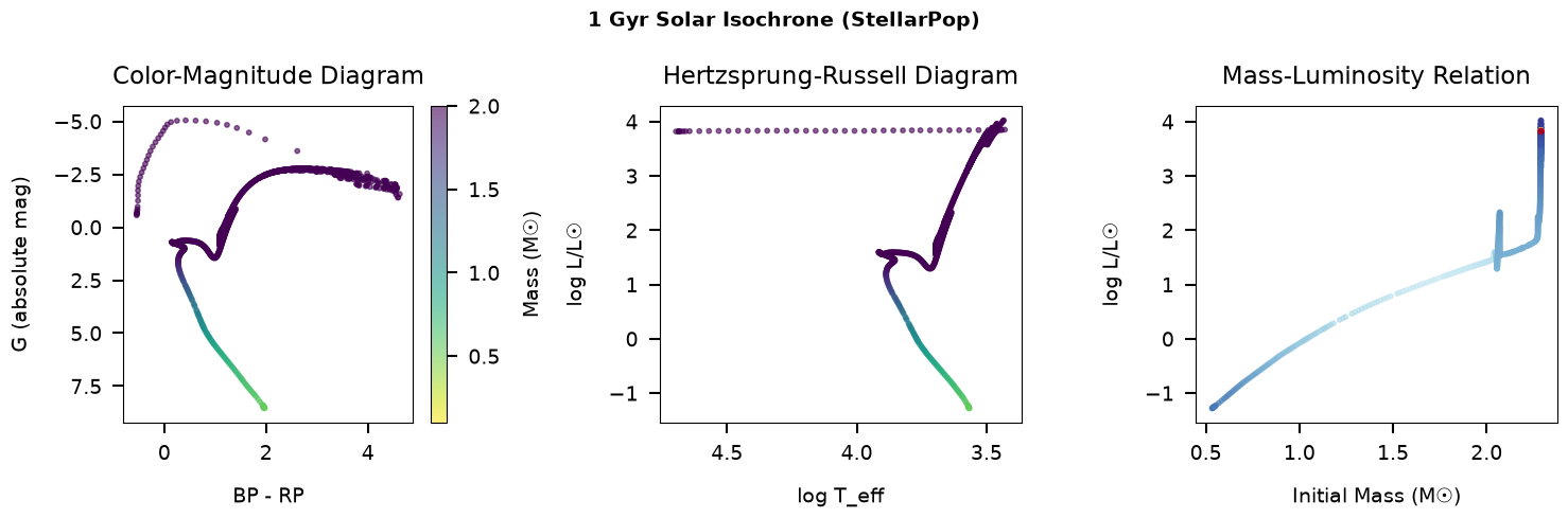
# Evaluate isochrone SEDs
print("Evaluating 1 Gyr solar metallicity isochrone...")

# Isochrone parameters
feh, afe, loga = 0.0, 0.0, 9.0  # Solar metallicity, 1 Gyr
av, rv, dist = 0.0, 3.32, 10.0   # 10 pc (absolute mags), no extinction

# Generate photometry for all EEP points along the isochrone
# Note: get_seds returns one SED per EEP point, not an IMF-sampled population
mags, params, binary_params = pop.get_seds(
    feh=feh, afe=afe, loga=loga,
    av=av, rv=rv, dist=dist,
    binary_fraction=0.0
)

# Filter to valid (finite) models
valid = np.all(np.isfinite(mags), axis=1) & np.isfinite(params['mini'])
print(f"Evaluated {len(mags)} EEP points, {valid.sum()} with valid photometry")
print(f"  Mass range: {params['mini'][valid].min():.2f} - {params['mini'][valid].max():.2f} M☉")

# Show magnitude statistics
print("\nMagnitude statistics (valid models at 10 pc):")
for i, f in enumerate(filt):
    vals = mags[valid, i]
    print(f"  {f}: {np.median(vals):.1f} (range {vals.min():.1f} to {vals.max():.1f}) mag")

Evaluating 1 Gyr solar metallicity isochrone...
Evaluated 1710 EEP points, 1206 with valid photometry
  Mass range: 0.53 - 2.29 M☉

Magnitude statistics (valid models at 10 pc):
  Gaia_G_MAW: -2.0 (range -5.0 to 8.6) mag
  Gaia_BP_MAWf: -0.1 (range -4.9 to 9.6) mag
  Gaia_RP_MAW: -3.3 (range -5.5 to 7.6) mag
  PS_g: 0.2 (range -5.0 to 9.9) mag
  PS_r: -0.8 (range -5.0 to 8.8) mag
  PS_i: -2.6 (range -5.1 to 8.0) mag

Show code cell source

Hide code cell source

# Visualize the isochrone
fig, axes = plt.subplots(1, 3, figsize=(15, 5))

# Panel 1: Gaia CMD
ax = axes[0]
bp_rp = mags[valid, 1] - mags[valid, 2]
g_mag = mags[valid, 0]
mini_valid = params['mini'][valid]

scatter = ax.scatter(bp_rp, g_mag, c=mini_valid, s=10,
                    cmap='viridis_r', vmin=0.1, vmax=2.0, alpha=0.6)
ax.set_xlabel('BP - RP')
ax.set_ylabel('G (absolute mag)')
ax.set_title('Color-Magnitude Diagram')
ax.invert_yaxis()
plt.colorbar(scatter, ax=ax, label='Mass (M☉)')

# Panel 2: HRD (with validity filter)
ax = axes[1]
hrd_valid = valid & np.isfinite(params['logt']) & np.isfinite(params['logl'])
ax.scatter(params['logt'][hrd_valid], params['logl'][hrd_valid],
          c=params['mini'][hrd_valid], s=10,
          cmap='viridis_r', vmin=0.1, vmax=2.0, alpha=0.6)
ax.set_xlabel('log T_eff')
ax.set_ylabel('log L/L☉')
ax.set_title('Hertzsprung-Russell Diagram')
ax.invert_xaxis()

# Panel 3: Mass-Luminosity relation
ax = axes[2]
ax.scatter(params['mini'][hrd_valid], params['logl'][hrd_valid],
          c=params['logt'][hrd_valid], s=10,
          cmap='RdYlBu_r', alpha=0.6)
ax.set_xlabel('Initial Mass (M☉)')
ax.set_ylabel('log L/L☉')
ax.set_title('Mass-Luminosity Relation')

plt.suptitle('1 Gyr Solar Isochrone (StellarPop)', fontsize=14, fontweight='bold')
plt.tight_layout()
save_figure(fig, 'stellarpop_isochrone')
plt.show()

  Saved: /mnt/c/Users/joshs/Dropbox/GitHub/brutus/tutorials/plots/tutorial_02/stellarpop_isochrone.png

Section 3: Isochrone Age Sequences

Stellar populations evolve with time as stars leave the main sequence. Let’s explore how isochrones change with age.

Age Effects

• Main sequence turnoff moves to lower masses with age

• Red giant branch develops for older populations

• Horizontal branch appears in old, metal-poor populations

• Color distribution becomes redder with age

Show code cell source

Hide code cell source

# Create age sequence plots
fig, axes = plt.subplots(1, 3, figsize=(15, 5))

# Age grid (log years)
ages = [6.6, 7.0, 8.0, 9.0, 9.5, 10.0]  # 4 Myr to 10 Gyr
age_labels = ['4 Myr', '10 Myr', '100 Myr', '1 Gyr', '3 Gyr', '10 Gyr']
colors = plt.cm.plasma(np.linspace(0.2, 0.9, len(ages)))

# Fixed metallicity
feh, afe = 0.0, 0.0
eep_grid = np.linspace(202, 808, 2000)

print("Generating age sequence...")

for loga, label, color in zip(ages, age_labels, colors):
    # Generate isochrone stellar parameters
    params_arr = iso.get_predictions(feh=feh, afe=afe, loga=loga, eep=eep_grid)
    params = {label: params_arr[:, i] for i, label in enumerate(iso.predictions)}
    
    # Get magnitudes using StellarPop
    mags, _, _ = pop.get_seds(feh=feh, afe=afe, loga=loga, eep=eep_grid, 
                               dist=10.0, binary_fraction=0.0)
    
    # Valid points
    valid = np.isfinite(params['mini']) & np.isfinite(mags[:, 0])
    
    # Panel 1: CMD
    bp_rp = mags[valid, 1] - mags[valid, 2]
    g_mag = mags[valid, 0]
    axes[0].plot(bp_rp, g_mag, color=color, lw=2, alpha=0.8, label=label)
    
    # Panel 2: HRD
    axes[1].plot(params['logt'][valid], params['logl'][valid],
                   color=color, lw=2, alpha=0.8)
    
    # Panel 3: Mass-Luminosity
    axes[2].plot(params['mini'][valid], params['logl'][valid],
                   color=color, lw=2, alpha=0.8)
    
    print(f"  {label}: {valid.sum()} valid points")

# Format all plots
axes[0].set_xlabel('BP - RP')
axes[0].set_ylabel('G magnitude (at 10 pc)')
axes[0].set_title('CMD Evolution')
axes[0].invert_yaxis()
axes[0].set_xlim(-0.5, 4.0)
axes[0].set_ylim(15, -5)
axes[0].legend(fontsize=8, loc='upper right')
axes[0].grid(True, alpha=0.3)

axes[1].set_xlabel('log T_eff')
axes[1].set_ylabel('log L/L☉')
axes[1].set_title('HRD Evolution')
axes[1].invert_xaxis()
axes[1].set_xlim(4.1, 3.3)
axes[1].set_ylim(-3, 5)
axes[1].grid(True, alpha=0.3)

axes[2].set_xlabel('Initial Mass (M☉)')
axes[2].set_ylabel('log L/L☉')
axes[2].set_title('Mass-Luminosity Relation')
axes[2].set_xscale('log')
axes[2].set_xlim(0.1, 10)
axes[2].set_ylim(-3, 5)
axes[2].grid(True, alpha=0.3)

plt.suptitle('Isochrone Age Sequences', fontsize=16, fontweight='bold')
plt.tight_layout()
save_figure(fig, 'age_sequences')
plt.show()

print("\nAge sequence effects demonstrated")

Generating age sequence...
  4 Myr: 1621 valid points

  10 Myr: 1999 valid points
  100 Myr: 2000 valid points
  1 Gyr: 1865 valid points
  3 Gyr: 1780 valid points
  10 Gyr: 1683 valid points

  Saved: /mnt/c/Users/joshs/Dropbox/GitHub/brutus/tutorials/plots/tutorial_02/age_sequences.png

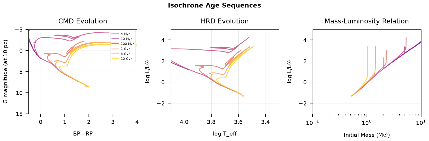
Age sequence effects demonstrated

Section 4: Metallicity Effects on Stellar Populations

Metallicity profoundly affects stellar populations, changing their colors, luminosities, and evolutionary timescales.

Metallicity Effects

• Metal-poor stars are bluer and hotter at fixed mass

• RGB position is sensitive to metallicity

• Main sequence width increases with metallicity spread

• Galactic components have distinct metallicity distributions

Show code cell source

Hide code cell source

# Create metallicity comparison plots
fig, axes = plt.subplots(1, 3, figsize=(15, 5))

# Metallicity grid
feh_values = [-2.0, -1.0, -0.5, 0.0, 0.3]
colors = plt.cm.RdYlBu_r(np.linspace(0.1, 0.9, len(feh_values)))

# Fixed age, use absolute magnitudes (10 pc)
loga, afe = 9.3, 0.0  # 2 Gyr
eep_grid = np.linspace(202, 808, 2000)

print("Generating metallicity sequence...")

for feh, color in zip(feh_values, colors):
    # Generate isochrone
    params_arr = iso.get_predictions(feh=feh, afe=afe, loga=loga, eep=eep_grid)
    params = {label: params_arr[:, i] for i, label in enumerate(iso.predictions)}
    
    # Get magnitudes at 10 pc (absolute)
    mags, _, _ = pop.get_seds(feh=feh, afe=afe, loga=loga, eep=eep_grid, 
                              dist=10.0, binary_fraction=0.0)
    
    # Valid points
    valid = np.isfinite(params['mini']) & np.all(np.isfinite(mags), axis=1)
    
    # Panel 1: Gaia CMD
    bp_rp = mags[valid, 1] - mags[valid, 2]
    g_mag = mags[valid, 0]
    axes[0].plot(bp_rp, g_mag, color=color, lw=2, alpha=0.8,
                   label=f'[Fe/H] = {feh:.1f}')
    
    # Panel 2: PS CMD
    g_ps = mags[valid, 3]  # PS g
    r_ps = mags[valid, 4]  # PS r
    axes[1].plot(g_ps - r_ps, g_ps, color=color, lw=2, alpha=0.8)
    
    # Panel 3: HRD
    hrd_valid = valid & np.isfinite(params['logt']) & np.isfinite(params['logl'])
    axes[2].plot(params['logt'][hrd_valid], params['logl'][hrd_valid],
                   color=color, lw=2, alpha=0.8)
    
    print(f"  [Fe/H] = {feh:+.1f}: {valid.sum()} valid points")

# Format plots
axes[0].set_xlabel('BP - RP')
axes[0].set_ylabel('G (absolute mag)')
axes[0].set_title('Gaia CMD')
axes[0].invert_yaxis()
axes[0].legend(fontsize=8)
axes[0].grid(True, alpha=0.3)

axes[1].set_xlabel('g - r (PS)')
axes[1].set_ylabel('g (absolute mag, PS)')
axes[1].set_title('Pan-STARRS CMD')
axes[1].invert_yaxis()
axes[1].grid(True, alpha=0.3)

axes[2].set_xlabel('log T_eff')
axes[2].set_ylabel('log L/L☉')
axes[2].set_title('HRD')
axes[2].invert_xaxis()
axes[2].grid(True, alpha=0.3)

plt.suptitle('Metallicity Effects on Isochrones', fontsize=16, fontweight='bold')
plt.tight_layout()
save_figure(fig, 'metallicity_populations')
plt.show()

print("\nMetallicity effects demonstrated")

Generating metallicity sequence...
  [Fe/H] = -2.0: 1728 valid points

  [Fe/H] = -1.0: 1741 valid points
  [Fe/H] = -0.5: 1754 valid points
  [Fe/H] = +0.0: 1829 valid points
  [Fe/H] = +0.3: 1775 valid points

  Saved: /mnt/c/Users/joshs/Dropbox/GitHub/brutus/tutorials/plots/tutorial_02/metallicity_populations.png

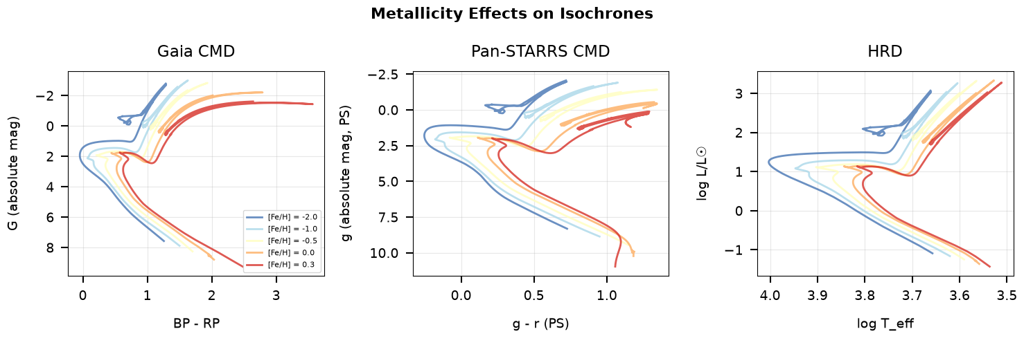
Metallicity effects demonstrated

Section 5: IMF Sampling and Mass Functions

The Initial Mass Function (IMF) determines the distribution of stellar masses in a population.

Kroupa IMF

brutus implements a Kroupa (2001) broken power-law IMF via logp_imf. This is a two-segment power law with a shallower slope at low masses (below the break mass) and a steeper slope at high masses:

• Low mass (M ≤ 0.5 M☉): α = 1.3

• High mass (M > 0.5 M☉): α = 2.3

The break mass, slopes, and mass limits are all configurable parameters of logp_imf.

Show code cell source

Hide code cell source

from brutus.priors.stellar import logp_imf

# Kroupa IMF: normalized mass function
fig, ax = plt.subplots(figsize=(8, 6))

mass_grid = np.logspace(-1, 2, 1000)

# Default Kroupa IMF (broken power law)
kroupa_lnp = logp_imf(mass_grid, alpha_low=1.3, alpha_high=2.3, mass_break=0.5)
kroupa_pdf = np.exp(kroupa_lnp)
kroupa_pdf /= np.trapz(kroupa_pdf, mass_grid)  # Normalize

ax.plot(mass_grid, kroupa_pdf, 'b-', lw=2.5, label=r'Kroupa ($\alpha_1$=1.3, $\alpha_2$=2.3)')

# Mark the break mass
break_mass = 0.5
break_idx = np.argmin(np.abs(mass_grid - break_mass))
ax.axvline(break_mass, color='gray', ls='--', lw=1, alpha=0.7, label=f'Break mass = {break_mass} M☉')

ax.set_xlabel('Mass (M☉)', fontsize=12)
ax.set_ylabel('Normalized probability density', fontsize=12)
ax.set_title('Kroupa IMF (brutus default)', fontsize=14, fontweight='bold')
ax.set_xscale('log')
ax.set_yscale('log')
ax.set_xlim(0.08, 100)
ax.legend(fontsize=11)
ax.grid(True, alpha=0.3)

save_figure(fig, 'imf_kroupa')
plt.show()

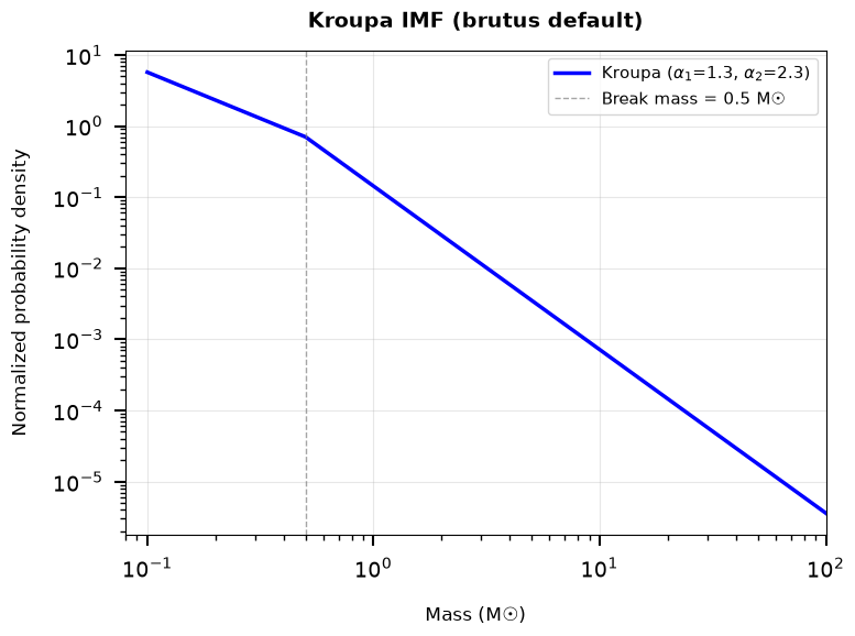
print('Kroupa IMF: Broken power law')
print(f'  Low-mass slope  (M <= {break_mass} M☉): alpha = 1.3')
print(f'  High-mass slope (M >  {break_mass} M☉): alpha = 2.3')
print(f'  Mass range: [{mass_grid[kroupa_pdf > 0].min():.2f}, {mass_grid[kroupa_pdf > 0].max():.1f}] M☉')

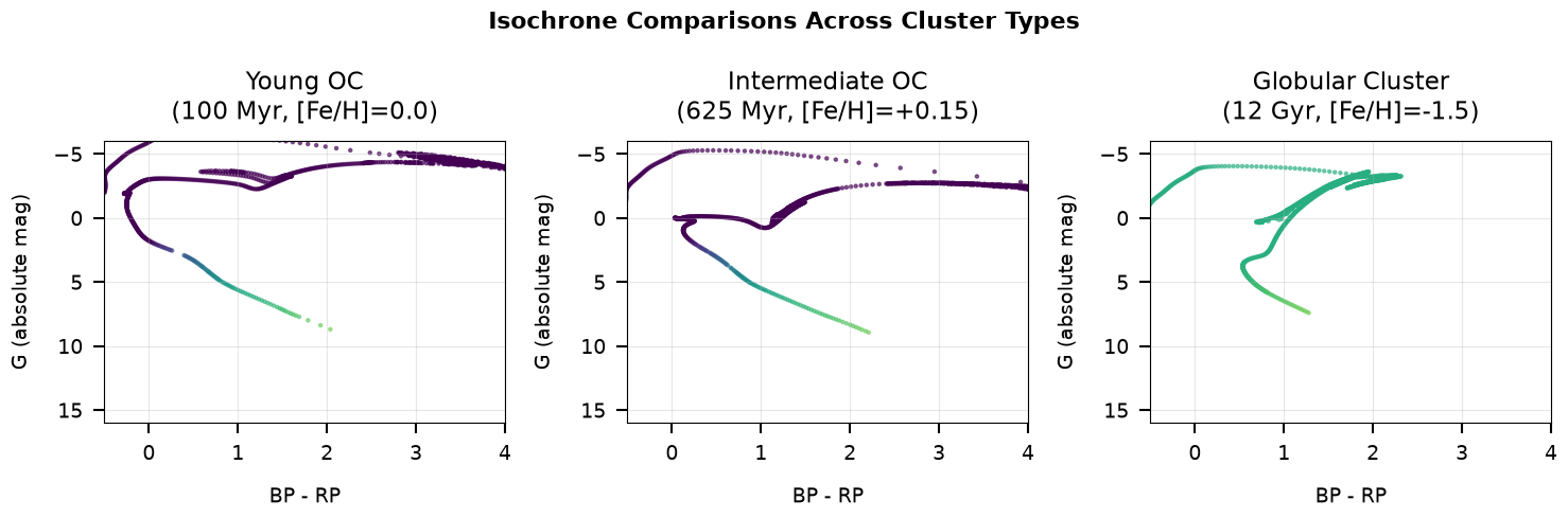
Section 6: Isochrone Comparisons Across Cluster Types

Different stellar environments have distinct ages, metallicities, and alpha enhancements. Let’s compare isochrones for three representative cluster types to see how these parameters affect the CMD and HRD.

# Extended filter set for multi-wavelength comparison
filt_full = filters.gaia + filters.ps[:3] + filters.tmass
pop_full = StellarPop(isochrone=iso, filters=filt_full, nnfile=nnfile, verbose=False)
print(f"Using extended filter set: {', '.join(filt_full)}")

# Generate isochrones for three different cluster types
# Use absolute magnitudes (dist=10 pc) so all are on the same scale
print("\nGenerating isochrones for different cluster types...\n")

# Cluster 1: Young open cluster (Pleiades-like)
print("  Young (100 Myr, solar)...")
mags1, params1, _ = pop_full.get_seds(
    feh=0.0, afe=0.0, loga=8.0,  # 100 Myr
    av=0.0, rv=3.32, dist=10.0,   # absolute magnitudes
    binary_fraction=0.0
)
valid1 = np.all(np.isfinite(mags1), axis=1)
print(f"    {valid1.sum()} valid EEP points")

# Cluster 2: Intermediate age (Hyades-like)
print("  Intermediate (625 Myr, slightly metal-rich)...")
mags2, params2, _ = pop_full.get_seds(
    feh=0.15, afe=0.0, loga=8.8,  # 625 Myr
    av=0.0, rv=3.32, dist=10.0,
    binary_fraction=0.0
)
valid2 = np.all(np.isfinite(mags2), axis=1)
print(f"    {valid2.sum()} valid EEP points")

# Cluster 3: Old globular cluster
# Note: We use afe=0.0 because the C3K neural network does not cover
# alpha-enhanced models. Real GCs are typically alpha-enhanced ([a/Fe]~0.3),
# but the NN returns NaN for any afe > 0.
print("  Old globular (12 Gyr, metal-poor)...")
mags3, params3, _ = pop_full.get_seds(
    feh=-1.5, afe=0.0, loga=10.08,  # 12 Gyr
    av=0.0, rv=3.32, dist=10.0,
    binary_fraction=0.0
)
valid3 = np.all(np.isfinite(mags3), axis=1)
print(f"    {valid3.sum()} valid EEP points")

Using extended filter set: Gaia_G_MAW, Gaia_BP_MAWf, Gaia_RP_MAW, PS_g, PS_r, PS_i, 2MASS_J, 2MASS_H, 2MASS_Ks

Generating isochrones for different cluster types...

  Young (100 Myr, solar)...
    1315 valid EEP points
  Intermediate (625 Myr, slightly metal-rich)...
    1273 valid EEP points
  Old globular (12 Gyr, metal-poor)...
    1199 valid EEP points

Show code cell source

Hide code cell source

# Create isochrone comparison visualization
fig, axes = plt.subplots(1, 3, figsize=(15, 5))

# Top row: Individual isochrone CMDs colored by mass
isochrones = [
    (mags1, params1, valid1, 'Young OC\n(100 Myr, [Fe/H]=0.0)'),
    (mags2, params2, valid2, 'Intermediate OC\n(625 Myr, [Fe/H]=+0.15)'),
    (mags3, params3, valid3, 'Globular Cluster\n(12 Gyr, [Fe/H]=-1.5)'),
]

# Common axis limits for fair comparison
common_xlim = (-0.5, 4.0)
common_ylim = (16, -6)

for idx, (mags, params, valid, title) in enumerate(isochrones):
    ax = axes[idx]
    
    bp_rp = mags[valid, 1] - mags[valid, 2]
    g_mag = mags[valid, 0]
    
    if np.any(valid):
        scatter = ax.scatter(bp_rp, g_mag,
                           c=params['mini'][valid],
                           s=5, cmap='viridis_r', vmin=0.1, vmax=2.0, alpha=0.6)
    else:
        ax.text(0.5, 0.5, 'No valid\nphotometry', transform=ax.transAxes,
                ha='center', va='center', fontsize=12, color='gray')
    
    ax.set_xlabel('BP - RP')
    ax.set_ylabel('G (absolute mag)')
    ax.set_title(title)
    ax.set_xlim(common_xlim)
    ax.set_ylim(common_ylim)
    ax.grid(True, alpha=0.3)

plt.suptitle('Isochrone Comparisons Across Cluster Types', fontsize=16, fontweight='bold')
plt.tight_layout()
save_figure(fig, 'cluster_isochrones')
plt.show()

print("\nIsochrone comparisons demonstrated")
print(f"  Total valid EEP points: {valid1.sum() + valid2.sum() + valid3.sum()}")

  Saved: /mnt/c/Users/joshs/Dropbox/GitHub/brutus/tutorials/plots/tutorial_02/cluster_isochrones.png

Isochrone comparisons demonstrated
  Total valid EEP points: 3787

Summary and Key Takeaways

This tutorial has covered stellar population modeling in brutus:

Key Classes

1. Isochrone: Models coeval stellar populations

   • Interpolates MIST isochrone tables

   • Returns stellar parameters for populations of given age/metallicity

   • Covers full range of stellar masses at each age

2. StellarPop: Generates synthetic populations with photometry

   • Combines Isochrone with neural network photometry

   • Handles binary populations

   • Applies extinction and distance effects

   • Enables realistic cluster simulations

Physical Effects

• Age: Determines turnoff mass and RGB properties

• Metallicity: Affects colors, luminosities, and evolution

• IMF: Controls the mass distribution and low-mass star counts

• Binaries: Create broader sequences and affect cluster dynamics

Applications

• Star cluster analysis and fitting

• Stellar population synthesis

• Galactic archaeology studies

• Calibration of stellar parameters

Next Steps

• Tutorial 3: Model Grids and Performance Optimization

• Tutorial 4: Galactic Priors and Population Synthesis

• Tutorial 5: Fitting Individual Sources with BruteForce

• Tutorial 6: Cluster Analysis and Bayesian Inference

print("Tutorial 2 Complete!")
print("="*60)
print("\nGenerated plots:")
for plot_file in sorted(plots_dir.glob('*.png')):
    print(f"  - {plot_file.name}")

Tutorial 2 Complete!
============================================================

Generated plots:
  - age_sequences.png
  - cluster_isochrones.png
  - imf_sampling.png
  - metallicity_populations.png
  - ps1_luminosity_function.png
  - stellarpop_isochrone.png