Tutorial 3: Model Grids and Performance#
This tutorial explores pre-computed model grids for fast SED generation and performance optimization.
Topics Covered#
GridGenerator for creating custom grids
StarGrid for fast SED lookups
Performance comparison: StarGrid vs StarEvolTrack
Loading and inspecting existing grids
Understanding reddening coefficients in grids
Reddened SED generation with
get_seds
Prerequisites#
This tutorial requires the following brutus data files:
MIST_1.2_EEPtrk.h5- MIST evolutionary tracksnn_c3k.h5- Neural network for bolometric correctionsgrid_mist_v9.h5(optional) - Pre-computed MIST gridgrid_bayestar_v5.h5(optional) - Pre-computed Bayestar grid
If you don’t have these files, run the optional download cell below.
# Optional: Download required data files (only needed if not already cached)
# This tutorial requires MIST evolutionary tracks, the C3K neural network,
# and optionally pre-computed model grids.
# Uncomment the lines below to download them.

# from brutus.data import fetch_tracks, fetch_nns, fetch_grids
# fetch_tracks()                  # ~60 MB  -- MIST evolutionary tracks
# fetch_nns()                     # ~50 MB  -- Neural network for bolometric corrections
# fetch_grids()                   # ~600 MB -- Pre-computed MIST grid (grid_mist_v9)
# fetch_grids('bayestar_v5')      # ~80 MB  -- Pre-computed Bayestar grid (grid_bayestar_v5)
# Imports and setup
import time
from pathlib import Path

import h5py
import numpy as np
import matplotlib.pyplot as plt
import warnings
warnings.filterwarnings('ignore')

from tutorial_utils import (
    setup_tutorial,
    find_brutus_data_file,
    save_figure as _save_fig,
    print_section,
)

info = setup_tutorial(3, title="Tutorial 03: Model Grids and Performance")
plots_dir = info['plot_dir']


def save_figure(fig, name):
    """Save figure to this tutorial's plot directory."""
    _save_fig(fig, 3, name)
Tutorial 03: Model Grids and Performance
========================================

Checking data requirements for Tutorial 3
=========================================
  Found: nn_c3k.h5
  Found: MIST_1.2_EEPtrk.h5
  Found: grid_mist_v9.h5
  Missing: grid_bayestar_v5.h5

  Missing 1 required file(s)
Section 1: Creating Model Grids with GridGenerator#
GridGenerator creates pre-computed model grids with reddening coefficients. This enables fast SED generation for large-scale fitting applications.
Key Concepts#
Grid parameters: Define the parameter space to sample (mass, metallicity, EEP, etc.)
Reddening coefficients: Store polynomial coefficients for fast extinction calculations
Reference distance: All grids use 1 kpc (1000 pc) reference distance
Storage format: HDF5 files with labels, parameters, and magnitude coefficients
from brutus.core import EEPTracks, GridGenerator
from brutus.data import filters

# Initialize components
print("Loading MIST tracks and neural networks...")
mistfile = find_brutus_data_file('MIST_1.2_EEPtrk.h5')
nnfile = find_brutus_data_file('nn_c3k.h5')

# Use subset of filters for speed
filt = filters.ps[:3] + filters.tmass[:2]  # g,r,i + J,H
print(f"Using filters: {', '.join(filt)}")

tracks = EEPTracks(mistfile=mistfile, verbose=False)
print("Loaded EEPTracks")
Loading MIST tracks and neural networks...
Using filters: PS_g, PS_r, PS_i, 2MASS_J, 2MASS_H
Loaded EEPTracks
# Create grid generator
print("Initializing GridGenerator...")
generator = GridGenerator(
    tracks=tracks,
    nnfile=nnfile,
    filters=filt,
    verbose=True
)

print("\nDefining grid parameters for a small demo grid...")

# Define small grid for demonstration
mini_grid = np.array([0.5, 0.8, 1.0, 1.5, 2.0])  # 5 masses
feh_grid = np.array([-1.0, 0.0, 0.3])  # 3 metallicities
eep_grid = np.linspace(300, 500, 21)  # 21 EEP points (MS only)
afe_grid = np.array([0.0])  # Single alpha
smf_grid = np.array([0.0])  # No binaries for speed

total_models = len(mini_grid) * len(feh_grid) * len(eep_grid) * len(afe_grid) * len(smf_grid)
print(f"\nGrid dimensions:")
print(f"  Masses: {len(mini_grid)} points")
print(f"  Metallicities: {len(feh_grid)} points")
print(f"  EEPs: {len(eep_grid)} points")
print(f"  Total models to generate: {total_models}")
Initializing GridGenerator...

Defining grid parameters for a small demo grid...

Grid dimensions:
  Masses: 5 points
  Metallicities: 3 points
  EEPs: 21 points
  Total models to generate: 315
Grid filters: [np.str_('PS_g'), np.str_('PS_r'), np.str_('PS_i'), np.str_('2MASS_J'), np.str_('2MASS_H')]
Initializing FastNN predictor...done!
Note: The sampling above is deliberately very sparse (5 masses, 3 metallicities, 21 EEP points) and is intended for illustration only. A grid this coarse is not suitable for science applications. For production-quality grid sampling strategies and parameter spacing, see Speagle et al. (2025).
# Generate the grid
print("\nGenerating model grid (this may take a minute)...")
start_time = time.time()

generator.make_grid(
    mini_grid=mini_grid,
    feh_grid=feh_grid,
    eep_grid=eep_grid,
    afe_grid=afe_grid,
    smf_grid=smf_grid,
    av_grid=np.linspace(0, 3, 4),  # For reddening coefficients
    rv_grid=np.array([3.32]),
    verbose=False
)

gen_time = time.time() - start_time
print(f"\nGrid generation complete in {gen_time:.1f} seconds")
print(f"  Models generated: {len(generator.grid_labels)}")
print(f"  Valid models: {generator.grid_sel.sum()}")
print(f"  Time per model: {gen_time/generator.grid_sel.sum()*1000:.1f} ms")
Generating model grid (this may take a minute)...
Grid generation complete in 0.3 seconds
  Models generated: 315
  Valid models: 235
  Time per model: 1.3 ms
# Save the demo grid
demo_grid_file = plots_dir / 'demo_grid.h5'
print(f"\nSaving demo grid to {demo_grid_file}")

with h5py.File(demo_grid_file, 'w') as f:
    # Save valid models only
    valid = generator.grid_sel
    f.create_dataset('labels', data=generator.grid_labels[valid])
    f.create_dataset('parameters', data=generator.grid_params[valid])
    f.create_dataset('mag_coeffs', data=generator.grid_seds[valid])

    # Add metadata
    f.attrs['filters'] = str(filt)
    f.attrs['reference_distance_pc'] = 1000.0
    f.attrs['rv'] = 3.32
    f.attrs['generation_time'] = gen_time
    f.attrs['n_models'] = valid.sum()

print(f"Saved {valid.sum()} models to HDF5 file")
print(f"  File size: {demo_grid_file.stat().st_size / 1024**2:.2f} MB")
Saving demo grid to /home/user/brutus/tutorials/plots/tutorial_03/demo_grid.h5
Saved 235 models to HDF5 file
  File size: 0.04 MB
Section 2: StarGrid for Fast SED Lookups#
StarGrid wraps a pre-computed grid of magnitude coefficients for interactive queries. Given stellar parameters (mass, EEP, metallicity), it interpolates the grid to return an SED at any extinction and distance.
Role in the brutus pipeline#
Interactive exploration:
StarGrid.get_seds()lets you query individual models by physical parameters via multi-linear interpolation.BruteForce fitting: The fitting engine accesses the raw
mag_coeffsarray directly, evaluating every grid model against each observed star in a single Numba-compiled pass — no per-model neural network call needed.Compact storage: Each model stores only 3 numbers per band (
mag,R,dR/dRv), so reddening at any(A_V, R_V)is a simple linear operation.
from brutus.core import StarGrid
from brutus.data import load_models

# Try to load a pre-computed grid
print("Loading pre-computed MIST grid...")

try:
    grid_file = find_brutus_data_file('grid_mist_v9.h5')
    filt_grid = filters.ps[:5] + filters.tmass  # PS + 2MASS

    models, labels, mask = load_models(grid_file, filters=filt_grid)
    print(f"Loaded {len(models):,} models")
    print(f"  Filters: {', '.join(filt_grid)}")

    # Initialize StarGrid (positional: models, models_labels)
    grid = StarGrid(models, labels, filters=filt_grid)
    print("StarGrid initialized")

    grid_available = True

except FileNotFoundError:
    print("Pre-computed grid not found")
    print("  Using demo grid from Section 1 instead...")

    # Load the demo grid we just created
    with h5py.File(demo_grid_file, 'r') as f:
        labels = f['labels'][:]
        models = f['mag_coeffs'][:]

    grid = StarGrid(models, labels, filters=filt)
    grid_available = False
Loading pre-computed MIST grid...
Reading entire dataset (49 filters) once...
Extracting 8 requested filters from memory: ['PS_g', 'PS_r', 'PS_i', 'PS_z', 'PS_y', '2MASS_J', '2MASS_H', '2MASS_Ks']
Dropping constant 'afe' label column (single-afe grid, afe=0)...
Loaded 613,530 models
  Filters: PS_g, PS_r, PS_i, PS_z, PS_y, 2MASS_J, 2MASS_H, 2MASS_Ks
Loaded StarGrid with 613,530 models, 8 filters, 8 labels
StarGrid initialized
# Test StarGrid performance
print("\nTesting StarGrid performance...")

# Generate 100 SEDs for timing
n_test = 100
start = time.time()

for _ in range(n_test):
    try:
        mag, params, _ = grid.get_seds(
            mini=1.0, feh=0.0, eep=400,
            av=0.5, rv=3.32, dist=1000.0
        )
    except:
        # May fail if parameters are out of grid range
        pass

grid_time = (time.time() - start) / n_test
print(f"  Average time per SED: {grid_time*1000:.2f} ms")

# Show example output
mag, params, _ = grid.get_seds(
    mini=1.0, feh=0.0, eep=400,
    av=0.0, rv=3.32, dist=1000.0
)

print(f"\nExample SED for 1 M_sun star at 1 kpc:")
for i, f in enumerate(grid.filters[:min(5, len(grid.filters))]):
    print(f"  {f}: {mag[i]:.2f} mag")

if isinstance(params, dict) and 'loga' in params:
    print(f"\nDerived parameters:")
    print(f"  Age: {10**(params['loga'])/1e9:.2f} Gyr")
    print(f"  log L/L_sun: {params.get('logl', 'N/A'):.2f}")
    print(f"  log Teff: {params.get('logt', 'N/A'):.2f}")
Testing StarGrid performance...
  Average time per SED: 30.80 ms

Example SED for 1 M_sun star at 1 kpc:
  PS_g: 14.62 mag
  PS_r: 14.28 mag
  PS_i: 14.19 mag
  PS_z: 14.18 mag
  PS_y: 14.18 mag

Derived parameters:
  Age: 6.75 Gyr
  log L/L_sun: 0.14
  log Teff: 3.77
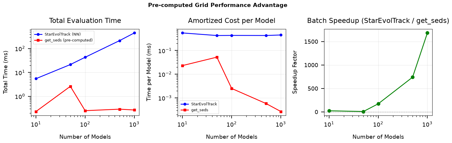
Section 3: Performance Comparison#
The real performance advantage of pre-computed grids shows up in
batch evaluation. During fitting, BruteForce applies reddening
to all grid models at once using the stored magnitude coefficients.
Each evaluation is a simple linear operation — 3 multiplies and 2 adds
per model per band, compiled with Numba — instead of an expensive
neural-network forward pass.
Below we compare:
StarEvolTrack: N individual on-the-fly SED evaluations (track interpolation + neural network per call)
get_sedson pre-computed coefficients: Applying reddening to N storedmag_coeffsin a single batch call
from brutus.core import StarEvolTrack, get_seds

# Setup
filt_test = filters.ps[:3] + filters.tmass[:2]
tracks = EEPTracks(mistfile=mistfile, verbose=False)
star_evol = StarEvolTrack(tracks=tracks, nnfile=nnfile, filters=filt_test, verbose=False)

# ------------------------------------------------------------------
# Compare: N individual StarEvolTrack calls  vs  one batch get_seds call
# This mirrors what BruteForce does — it never calls StarGrid.get_seds()
# for single-point lookups. Instead it passes the entire mag_coeffs array
# to _get_seds() in one Numba-compiled pass.
# ------------------------------------------------------------------
rng = np.random.default_rng(42)
test_minis = rng.uniform(0.5, 2.0, 2000)
test_fehs = rng.uniform(-1, 0.3, 2000)
test_eeps = rng.uniform(300, 500, 2000)

# Warm up Numba JIT (first call compiles the function)
if grid_available:
    _ = get_seds(models[:2], av=np.array([0.5, 1.0]), rv=np.array([3.32, 3.32]))

n_values = [10, 50, 100, 500, 1000]
evol_times = []
grid_times = []

print("Per-model cost: StarEvolTrack (NN) vs get_seds (pre-computed coefficients)\n")

for n in n_values:
    # Method 1: N individual StarEvolTrack.get_seds() calls
    #   Each call runs: track interpolation -> NN forward pass -> extinction
    start = time.time()
    for i in range(n):
        try:
            star_evol.get_seds(mini=test_minis[i], feh=test_fehs[i],
                               eep=test_eeps[i], dist=1000.0)
        except Exception:
            pass
    t_evol = time.time() - start
    evol_times.append(t_evol)

    # Method 2: Single get_seds() call on N pre-computed mag_coeffs
    #   Just applies: m = mag + Av * (R + Rv * dR/dRv) for all N models
    if grid_available:
        idx = rng.choice(len(models), n, replace=False)
        batch_coeffs = models[idx]  # (N, Nfilt, 3)
        av_arr = rng.uniform(0, 2, n)
        rv_arr = np.full(n, 3.32)

        start = time.time()
        _ = get_seds(batch_coeffs, av=av_arr, rv=rv_arr)
        t_grid = time.time() - start
        grid_times.append(t_grid)

        speedup = t_evol / t_grid if t_grid > 0 else float('inf')
        print(f"  N={n:5d}:  StarEvolTrack = {t_evol*1000:8.1f} ms,  "
              f"get_seds = {t_grid*1000:8.3f} ms  "
              f"(batch {speedup:.0f}x faster)")
    else:
        grid_times.append(None)
        print(f"  N={n:5d}:  StarEvolTrack = {t_evol*1000:8.1f} ms")

print("\nStarEvolTrack cost is dominated by the neural-network forward pass")
print("and Python-level track interpolation on each call.")
print("get_seds applies a simple linear formula to pre-computed coefficients,")
print("so the batch cost grows negligibly with N.")
Per-model cost: StarEvolTrack (NN) vs get_seds (pre-computed coefficients)

  N=   10:  StarEvolTrack =      5.5 ms,  get_seds =    0.232 ms  (batch 24x faster)
  N=   50:  StarEvolTrack =     21.4 ms,  get_seds =    2.624 ms  (batch 8x faster)
  N=  100:  StarEvolTrack =     43.3 ms,  get_seds =    0.251 ms  (batch 172x faster)
N= 500: StarEvolTrack = 214.9 ms, get_seds = 0.291 ms (batch 739x faster)
  N= 1000:  StarEvolTrack =    451.7 ms,  get_seds =    0.268 ms  (batch 1683x faster)

StarEvolTrack cost is dominated by the neural-network forward pass
and Python-level track interpolation on each call.
get_seds applies a simple linear formula to pre-computed coefficients,
so the batch cost grows negligibly with N.
Saved: /home/user/brutus/tutorials/plots/tutorial_03/performance_comparison.png
Pre-computed grids trade memory for speed: store mag_coeffs once,
then evaluate any (Av, Rv, dist) combination with trivial arithmetic.
Section 4: Working with Existing Grids#
Brutus provides pre-computed grids for common use cases. Let’s explore the available grids and their properties.
Available Grids#
grid_mist_v9.h5: Full MIST stellar evolution models
grid_bayestar_v5.h5: Empirical Pan-STARRS models for dust mapping
Note: These pre-computed grids have much denser sampling than the demo grid created above. For example, the MIST grid uses fine spacing in mass (typically ~0.01 M\u2609), EEP (~1\u20135), and metallicity (~0.05 dex). Inspect the grid metadata (shown below) for exact parameter ranges and spacing.
# Check for available grids
grids_to_check = [
    ('grid_mist_v9.h5', 'MIST v9', 'Full MIST stellar evolution models'),
    ('grid_bayestar_v5.h5', 'Bayestar v5', 'Empirical Pan-STARRS models'),
]

loaded_grids = []

for (filename, name, description) in grids_to_check:
    print(f"\n{name}: {description}")
    print("-" * 50)

    try:
        filepath = Path(find_brutus_data_file(filename))

        # Open to inspect
        with h5py.File(filepath, 'r') as f:
            print(f"  File: {filename}")
            print(f"  Size: {filepath.stat().st_size / 1024**2:.1f} MB")
            print(f"  Keys: {list(f.keys())}")

            if 'labels' in f:
                grid_labels = f['labels'][:]
                print(f"  Number of models: {len(grid_labels):,}")
                print(f"  Label fields: {grid_labels.dtype.names}")

                # Get parameter ranges
                if 'mini' in grid_labels.dtype.names:
                    print(f"  Mass range: {grid_labels['mini'].min():.2f} - {grid_labels['mini'].max():.2f} M\u2609")
                if 'feh' in grid_labels.dtype.names:
                    print(f"  [Fe/H] range: {grid_labels['feh'].min():.2f} - {grid_labels['feh'].max():.2f}")
                if 'Mr' in grid_labels.dtype.names:
                    print(f"  M_r range: {grid_labels['Mr'].min():.1f} - {grid_labels['Mr'].max():.1f}")

            if 'mag_coeffs' in f:
                mags = f['mag_coeffs']
                # mag_coeffs can be a structured array (filter names as fields,
                # each with 3 coefficients) or a regular (N, Nfilt, 3) array.
                if mags.dtype.names:
                    n_filters = len(mags.dtype.names)
                    print(f"  Magnitude coefficients: {len(mags):,} models x {n_filters} filters x 3 coefficients")
                    print(f"  Filter names: {', '.join(mags.dtype.names[:5])}...")
                else:
                    print(f"  Magnitude array shape: {mags.shape}")

            # Check metadata
            if f.attrs:
                print("  Metadata:")
                for key in list(f.attrs.keys())[:5]:
                    print(f"    {key}: {f.attrs[key]}")

            loaded_grids.append((name, grid_labels, filename))

    except FileNotFoundError:
        print(f"  [Not found - optional file]")
MIST v9: Full MIST stellar evolution models
--------------------------------------------------
  File: grid_mist_v9.h5
  Size: 744.3 MB
  Keys: ['labels', 'mag_coeffs', 'parameters']
  Number of models: 613,530
  Label fields: ('mini', 'eep', 'feh', 'afe', 'smf')
  Mass range: 0.50 - 2.00 M☉
  [Fe/H] range: -3.00 - 0.45
  Magnitude coefficients: 613,530 models x 49 filters x 3 coefficients
  Filter names: Gaia_G_MAW, Gaia_BP_MAWf, Gaia_RP_MAW, SDSS_u, SDSS_g...

Bayestar v5: Empirical Pan-STARRS models
--------------------------------------------------
  [Not found - optional file]
Section 5: Understanding Reddening Coefficients#
Model grids store reddening coefficients to enable fast extinction calculations without needing to re-evaluate the neural network for each value of $A_V$.
Reddening Parameterization#
For each model and filter, the mag_coeffs array stores 3 values:
mag: The unreddened apparent magnitude at the reference distance (1 kpc)R: The reddening vector component at $R_V = 0$dR/dR_V: The change in the reddening vector per unit $R_V$
The reddened magnitude in each band is then:
$$m_\lambda = \text{mag} + A_V \times (R + R_V \times dR/dR_V)$$
This parameterization captures the full wavelength-dependent extinction law with only 3 stored numbers per model per band, enabling fast evaluation for any combination of $A_V$ and $R_V$.
# Demonstrate the reddening coefficient structure
print("Reddening Coefficient Structure in brutus Grids\n")

print("Each model and filter stores 3 coefficients: [mag, R, dR/dRv]")
print()
print("  mag   : unreddened magnitude at 1 kpc reference distance")
print("  R     : reddening vector component at Rv=0")
print("  dR/dRv: change in reddening vector per unit Rv")
print()
print("Reddened magnitude:")
print("  m_lambda = mag + Av * (R + Rv * dR/dRv)")
print()
print("Benefits of this parameterization:")
print("  - Fast evaluation for any (Av, Rv) combination")
print("  - No neural network re-evaluation needed")
print("  - Linear in Av, linear in Rv")
print("  - Only 3 numbers per model per band")
print()

# Show example from the demo grid
# grid_seds is a structured array: each field is a filter name with shape (3,)
seds = generator.grid_seds
seds_fields = seds.dtype.names
print(f"Example from demo grid:")
print(f"  {len(seds)} models, {len(seds_fields)} filters, 3 coefficients each")

# Pick a valid model
valid_idx = np.where(generator.grid_sel)[0][0]
print(f"\nModel {valid_idx} coefficients:")
for fname in seds_fields:
    coeffs = seds[valid_idx][fname]
    print(f"  {fname}: mag={coeffs[0]:.2f}, R={coeffs[1]:.4f}, dR/dRv={coeffs[2]:.4f}")
Reddening Coefficient Structure in brutus Grids

Each model and filter stores 3 coefficients: [mag, R, dR/dRv]

  mag   : unreddened magnitude at 1 kpc reference distance
  R     : reddening vector component at Rv=0
  dR/dRv: change in reddening vector per unit Rv

Reddened magnitude:
  m_lambda = mag + Av * (R + Rv * dR/dRv)

Benefits of this parameterization:
  - Fast evaluation for any (Av, Rv) combination
  - No neural network re-evaluation needed
  - Linear in Av, linear in Rv
  - Only 3 numbers per model per band

Example from demo grid:
  315 models, 5 filters, 3 coefficients each

Model 0 coefficients:
  PS_g: mag=18.82, R=0.5640, dR/dRv=0.1699
  PS_r: mag=17.88, R=0.4111, dR/dRv=0.1238
  PS_i: mag=17.46, R=0.2871, dR/dRv=0.0865
  2MASS_J: mag=16.09, R=0.1091, dR/dRv=0.0329
  2MASS_H: mag=15.44, R=0.0672, dR/dRv=0.0202
Section 6: Reddened SED Generation with get_seds#
The get_seds function is the core utility for applying dust reddening to
pre-computed magnitude coefficients. Each model stores a compact representation
of how its photometry changes with extinction:
mag_coeffs array has shape (Nmodels, Nbands, 3) where the 3 coefficients are:
mag(index 0): The unreddened apparent magnitude at the reference distance (1 kpc).R(index 1): The reddening vector component atR(V) = 0.dR/dRv(index 2): The change in the reddening vector per unitR(V).
The reddened magnitude in each band is computed as:
$$m_\lambda = \text{mag} + A_V \times (R + R_V \times dR/dR_V)$$
This parameterization captures the full wavelength-dependent extinction law
with only 3 stored numbers per model per band, enabling extremely fast
evaluation for any combination of A(V) and R(V).
# Demonstrate the get_seds function for applying reddening to mag_coeffs
try:
    from brutus.core import get_seds

    # --- Build synthetic mag_coeffs (Nmodels, Nbands, 3) ---
    # If a grid was loaded earlier we grab a few rows; otherwise we
    # construct a small illustrative array by hand.
    try:
        # Use the first 5 models from the loaded grid
        sample_coeffs = models[:5].copy()
        band_labels = filt_grid if grid_available else filt
        print("Using mag_coeffs from the loaded grid (first 5 models).")
    except Exception:
        # Create synthetic coefficients for 5 "models" and 5 "bands"
        Nmodels, Nbands = 5, 5
        band_labels = ['g', 'r', 'i', 'J', 'H']
        sample_coeffs = np.zeros((Nmodels, Nbands, 3))
        # Unreddened magnitudes (index 0) -- typical main-sequence values
        sample_coeffs[:, :, 0] = np.array([[18.0, 17.2, 16.8, 15.5, 15.0],
                                            [16.5, 15.8, 15.4, 14.3, 13.9],
                                            [15.0, 14.5, 14.2, 13.4, 13.1],
                                            [20.0, 19.0, 18.5, 17.0, 16.5],
                                            [22.0, 21.0, 20.5, 19.0, 18.5]])
        # R (reddening at Rv=0, index 1) -- roughly A_lambda / A_V at Rv=0
        sample_coeffs[:, :, 1] = np.array([1.20, 0.87, 0.68, 0.29, 0.18])
        # dR/dRv (index 2) -- change per unit Rv
        sample_coeffs[:, :, 2] = np.array([0.32, 0.24, 0.18, 0.08, 0.05])
        print("Created synthetic mag_coeffs for 5 models x 5 bands.")

    print(f"  mag_coeffs shape: {sample_coeffs.shape}")
    print(f"  Interpretation: (Nmodels={sample_coeffs.shape[0]}, "
          f"Nbands={sample_coeffs.shape[1]}, coeffs=[mag, R, dR/dRv])")

    # --- Call get_seds at different extinction levels ---
    seds_av0 = get_seds(sample_coeffs, av=0.0)
    seds_av1 = get_seds(sample_coeffs, av=1.0, rv=3.3)
    seds_av2 = get_seds(sample_coeffs, av=2.0, rv=3.3)

    print(f"\nUnreddened SEDs (A_V=0)  shape: {seds_av0.shape}")
    print(f"Reddened SEDs  (A_V=1)  shape: {seds_av1.shape}")
    print(f"Reddened SEDs  (A_V=2)  shape: {seds_av2.shape}")

    print(f"\nModel 0 magnitudes across bands:")
    header = "  {:>8s}".format("Band") + "    A_V=0    A_V=1    A_V=2"
    print(header)
    for j in range(min(sample_coeffs.shape[1], len(band_labels))):
        label = band_labels[j] if j < len(band_labels) else f"band_{j}"
        print(f"  {label:>8s}   {seds_av0[0, j]:7.3f}  {seds_av1[0, j]:7.3f}  "
              f"{seds_av2[0, j]:7.3f}")

    get_seds_available = True

except Exception as e:
    print(f"Could not run get_seds demo: {e}")
    get_seds_available = False
Using mag_coeffs from the loaded grid (first 5 models).
  mag_coeffs shape: (5, 8, 3)
  Interpretation: (Nmodels=5, Nbands=8, coeffs=[mag, R, dR/dRv])

Unreddened SEDs (A_V=0)  shape: (5, 8)
Reddened SEDs  (A_V=1)  shape: (5, 8)
Reddened SEDs  (A_V=2)  shape: (5, 8)

Model 0 magnitudes across bands:
      Band    A_V=0    A_V=1    A_V=2
      PS_g    18.197   19.344   20.491
      PS_r    17.573   18.407   19.242
      PS_i    17.286   17.865   18.443
      PS_z    17.150   17.591   18.032
      PS_y    17.074   17.433   17.791
   2MASS_J    16.142   16.371   16.600
   2MASS_H    15.678   15.818   15.957
  2MASS_Ks    15.567   15.653   15.739
Summary and Key Takeaways#
This tutorial has covered model grids and performance optimization in brutus:
Key Classes#
GridGenerator: Creates pre-computed model grids
Samples parameter space systematically
Computes reddening coefficients (
mag,R,dR/dRvper band)Saves to HDF5 format
StarGrid: Interactive SED queries via grid interpolation
Multi-linear interpolation for any point in parameter space
Supports all extinction and distance effects
get_seds: Batch reddening applicationApplies
m = mag + Av * (R + Rv * dR/dRv)to pre-computed coefficientsOrders of magnitude faster than per-model neural network evaluation
Used internally by
BruteForcefor fitting
Performance Insights#
Speed: Pre-computed grids avoid per-model neural network calls during fitting
Reddening: 3-coefficient parameterization enables fast evaluation at any
(Av, Rv)Scalability: Grids enable fitting millions of stars with
BruteForce
Recommended Workflows#
Exploration: Use
StarEvolTrackfor flexibility at individual pointsProduction: Generate custom grid for your parameter space with
GridGeneratorLarge surveys: Use pre-computed grids (MIST, Bayestar) with
BruteForce
Next Steps#
Tutorial 4: Galactic Priors and Population Synthesis
Tutorial 5: Fitting Individual Sources with BruteForce
Tutorial 6: Cluster Analysis and Population Fitting
Tutorial 7: 3D Dust Mapping
print("Tutorial 3 Complete!")
print("="*60)
print("\nGenerated files and plots:")
for file in sorted(plots_dir.glob('*')):
    size = file.stat().st_size / 1024**2 if file.suffix == '.h5' else file.stat().st_size / 1024
    unit = 'MB' if file.suffix == '.h5' else 'KB'
    print(f"  - {file.name} ({size:.1f} {unit})")
Tutorial 3 Complete!
============================================================

Generated files and plots:
  - demo_grid.h5 (0.0 MB)
  - existing_grids.png (184.2 KB)
  - get_seds_av_comparison.png (169.2 KB)
  - get_seds_reddening_vectors.png (192.1 KB)
  - grid_resolution.png (241.4 KB)
  - performance_comparison.png (127.7 KB)
  - reddening_coefficients.png (142.2 KB)