Tutorial 4: Galactic Priors and Models#
This tutorial explores the prior probability distributions used in brutus for modeling stars in the Milky Way context.
Topics Covered#
Galactic structure priors (thin disk, thick disk, halo)
3D dust priors with Bayestar
Distance and parallax priors
Prior factorization and combination
Metallicity and age-metallicity priors
Prerequisites#
This tutorial requires the following brutus data files:
nn_c3k.h5- Neural network for bolometric correctionsMIST_1.2_iso_vvcrit0.0.h5- MIST isochronesbayestar2019_v1.h5(optional) - Bayestar dust map
If you don’t have these files, run the optional download cell below.
# Optional: Download required data files (only needed if not already cached)
# Uncomment the lines below to download them.

# from brutus.data import fetch_isos, fetch_nns, fetch_dustmaps
# fetch_isos()       # ~200 MB -- MIST isochrones
# fetch_nns()        # ~50 MB  -- Neural network for bolometric corrections
# fetch_dustmaps()   # ~2 GB   -- Bayestar 3D dust map (optional)
# Imports and setup
import numpy as np
import matplotlib.pyplot as plt
from pathlib import Path
import warnings
warnings.filterwarnings('ignore')

from tutorial_utils import (
    setup_tutorial,
    find_brutus_data_file,
    save_figure as _save_fig,
    print_section,
)

info = setup_tutorial(4, title="Tutorial 04: Galactic Priors and Models")
plots_dir = info['plot_dir']


def save_figure(fig, name):
    """Save figure to this tutorial's plot directory."""
    _save_fig(fig, 4, name)
Tutorial 04: Galactic Priors and Models
=======================================

Checking data requirements for Tutorial 4
=========================================
  Found: nn_c3k.h5
  Found: MIST_1.2_iso_vvcrit0.0.h5
  Found: bayestar2019_v1.h5

  All required files available
Section 1: Galactic Structure - 3D Density Models#
The Galaxy has distinct structural components with different spatial distributions, ages, and metallicities.
Components#
Thin Disk: Scale height ~300 pc, young/metal-rich stars
Thick Disk: Scale height ~900 pc, old/metal-poor stars
Halo: Power-law profile, very old/metal-poor stars
Each component dominates at different Galactic latitudes and distances.
Computing Galactic priors for different sightlines...
Saved: /home/user/brutus/tutorials/plots/tutorial_04/galactic_structure.png
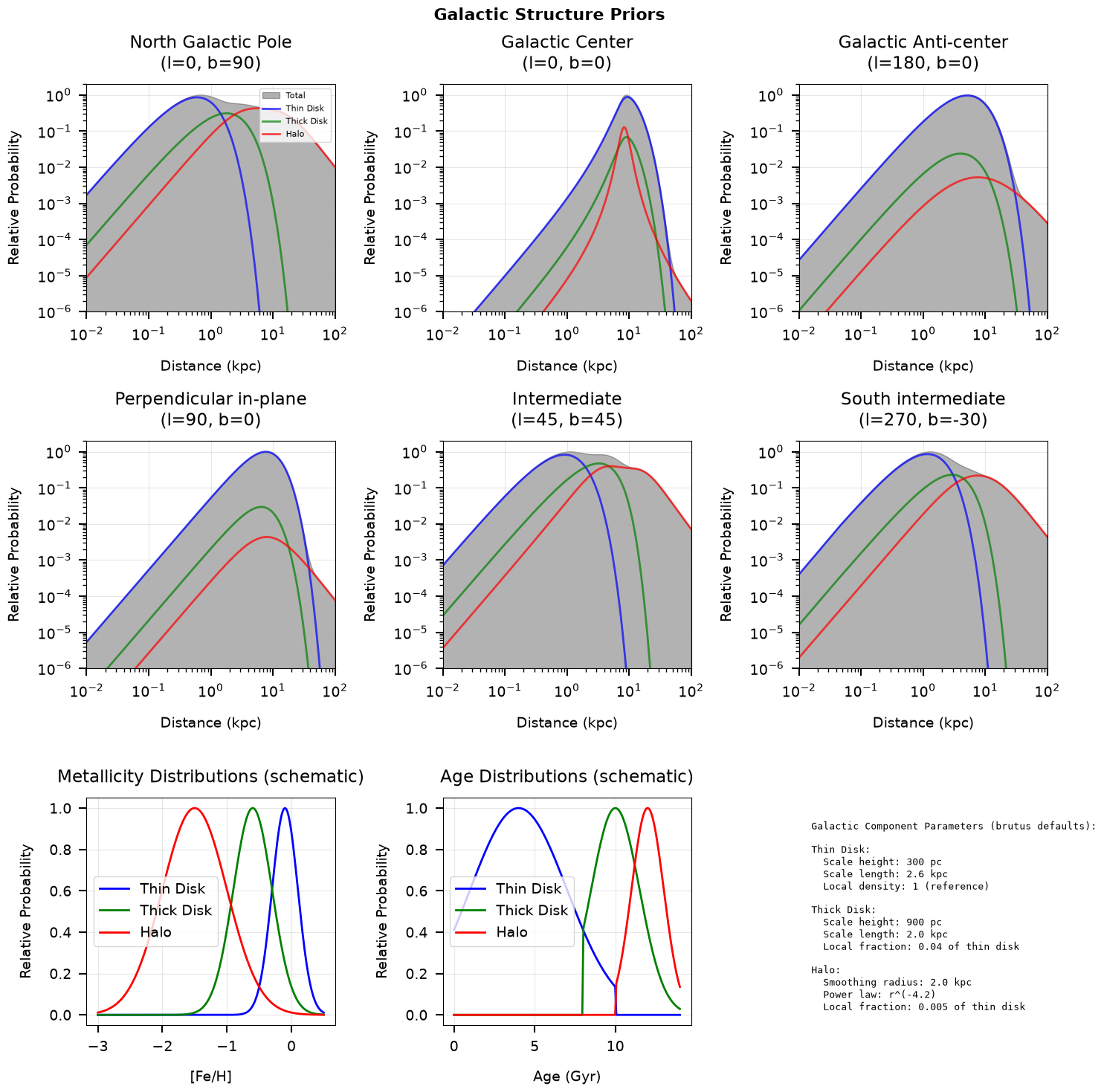
Galactic structure prior demonstrations complete
  Key points:
  - Thin disk dominates at low latitudes
  - Halo becomes important at high latitudes and large distances
  - Each component has distinct [Fe/H] and age distributions
Section 2: 3D Dust Extinction#
The Bayestar class in brutus.dust provides distance-resolved extinction estimates. For any Galactic sightline, it returns A(V) mean and standard deviation as a function of distance, based on Pan-STARRS and 2MASS photometry.
Key properties:
120 distance bins from ~0.06 to ~60 kpc at ~7 arcmin HEALPix resolution
A(V) uncertainty grows with distance
Extinction concentrated near the Galactic plane
Returns uniform prior for sightlines outside map coverage
By default, queries also honor the map’s per-pixel reliability metadata: distance bins outside a pixel’s reliable distance range, and pixels whose fits did not converge, are returned as NaN (pass
Bayestar(..., apply_reliability_mask=False)for the raw, unmasked profiles)
The logp_extinction function wraps Bayestar queries to provide a Gaussian log-prior on A(V) at a given distance and sky position, truncated and renormalized over the fitted A(V) range (avlim).
Coverage limitations: Bayestar is based on Pan-STARRS photometry and has no coverage in the southern sky below declination ~ -30 degrees. Coverage is also incomplete near the Galactic center due to extreme crowding and extinction. For sightlines outside the map footprint — and, with the default reliability masking, for distance bins the map flags as unreliable —
logp_extinctionreturns a uniform (uninformative) prior.
Loaded Bayestar dust map from /root/.cache/astro-brutus/bayestar2019_v1.h5

Querying Bayestar dust map for different sightlines...
  (l=  0, b= +0): max A(V) = 1.38
  (l= 90, b= +0): max A(V) = 2.81
  (l=180, b= +0): max A(V) = 2.93
  (l= 45, b=+30): max A(V) = 0.10
  (l=  0, b=+90): max A(V) = 0.01
Saved: /home/user/brutus/tutorials/plots/tutorial_04/dust_extinction.png
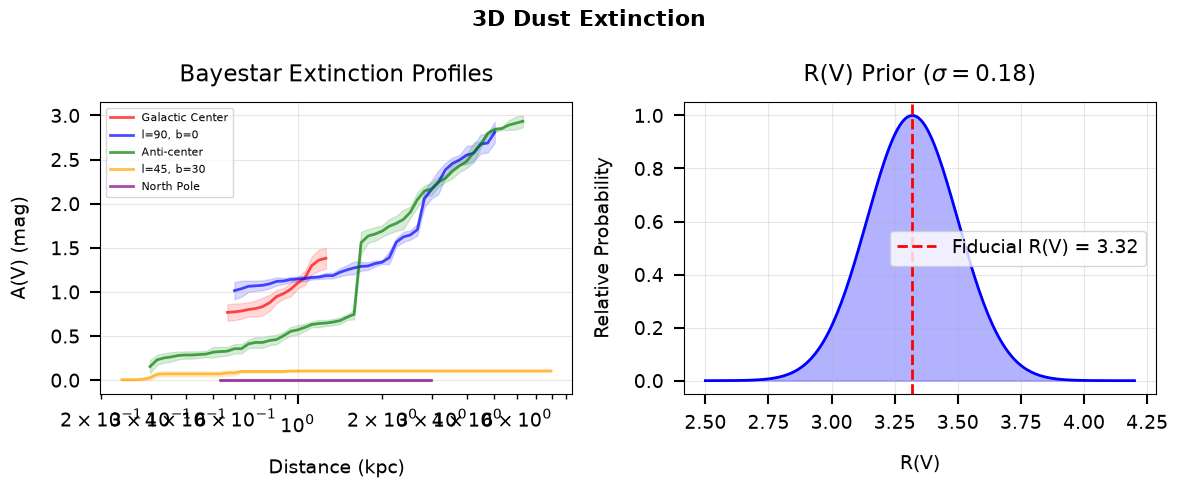
3D dust extinction demonstrations complete
  Key points:
  - Extinction increases with distance
  - Higher extinction near Galactic plane
  - Uncertainties grow with distance
Section 3: Parallax and Distance Priors#
Parallax measurements from Gaia constrain stellar distances. The logp_parallax function provides a Gaussian log-prior on the model parallax given an observed parallax and its uncertainty.
Key concepts:
Non-linear transformation: d = 1/pi leads to asymmetric distance uncertainties
Lutz-Kelker bias: Volume effects bias distance estimates outward at low signal-to-noise
Saved: /home/user/brutus/tutorials/plots/tutorial_04/parallax_distance.png
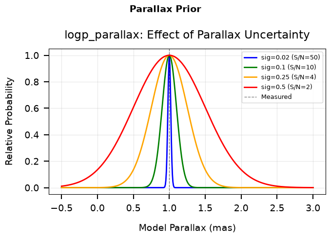
Parallax prior demonstration complete
  Key points:
  - logp_parallax provides Gaussian prior on observed parallax
  - Width of prior controlled by measurement uncertainty
  - At low S/N, the prior becomes broad and asymmetric in distance space
Section 4: Prior Factorization and Combination#
The complete prior in brutus combines all components multiplicatively, with proper factorization based on conditional independence.
Prior Factorization#
The full prior can be written as:
P(θ) = P(M) × P(d,Z,τ|l,b) × P(A_V|d,l,b) × P(π_obs|d)
Where:
P(M): IMF prior on stellar mass
P(d,Z,τ|l,b): Galactic structure prior (distance, metallicity, age given position)
P(A_V|d,l,b): 3D dust prior (extinction given distance and position)
P(π_obs|d): Parallax likelihood (observed parallax given true distance)
Saved: /home/user/brutus/tutorials/plots/tutorial_04/prior_combination.png
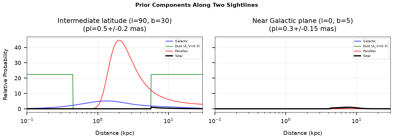
Prior combination demonstrations complete
  Key points:
  - Priors combine multiplicatively
  - Each component provides independent constraints
  - Dust prior uses logp_extinction with distance-resolved Bayestar map
  - Different sightlines show different prior shapes
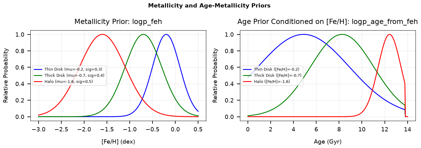
Section 5: Metallicity and Age-Metallicity Priors#
Beyond Galactic structure, brutus provides priors on stellar metallicity and an age-metallicity relation that encodes the observed correlation between stellar age and chemical enrichment.
Metallicity Prior: logp_feh#
The metallicity prior is a simple Gaussian parameterized by a mean and dispersion, with typical values for each Galactic component:
Thin disk:
feh_mean = -0.2,feh_sigma = 0.3Thick disk:
feh_mean = -0.7,feh_sigma = 0.4Halo:
feh_mean = -1.6,feh_sigma = 0.5
Age-Metallicity Relation: logp_age_from_feh#
The age prior is conditioned on metallicity through a logistic age-metallicity relation: metal-poor stars are preferentially older, while metal-rich stars are preferentially younger. The mean age and its dispersion are both functions of feh_mean, with ages drawn from a truncated normal distribution bounded by physically reasonable limits.
Saved: /home/user/brutus/tutorials/plots/tutorial_04/feh_age_priors.png
Metallicity & age-metallicity prior demonstrations complete
  Key points:
  - logp_feh is a Gaussian prior on [Fe/H] with component-specific means
  - logp_age_from_feh encodes the age-metallicity relation:
    metal-poor populations are preferentially older
  - The age dispersion narrows for metal-rich (younger) populations
Summary and Key Takeaways#
This tutorial has covered the prior probability distributions used in brutus:
Key Priors#
Galactic Structure: 3D spatial distribution
Thin disk: Young, metal-rich, low scale height
Thick disk: Old, metal-poor, high scale height
Halo: Very old, very metal-poor, power-law
Dust Maps: 3D extinction (Bayestar)
Provides A(V) as function of distance
Higher extinction in Galactic plane
Uncertainties increase with distance
Parallax: Distance constraints from Gaia
Non-linear parallax-distance transformation
Lutz-Kelker bias pushes distances outward
Metallicity & Age: Chemical evolution
Gaussian [Fe/H] priors per Galactic component
Age-metallicity relation encodes enrichment history
Prior Factorization#
The full prior combines multiplicatively:
P(theta) = P(M) x P(d,Z,tau|l,b) x P(A_V|d,l,b) x P(pi_obs|d)
Components are independent given position and observables.
Next Steps#
Tutorial 5: Fitting Individual Stars with BruteForce
Tutorial 6: Cluster Analysis and Population Fitting
Tutorial 7: 3D Dust Mapping
print("Tutorial 4 Complete!")
print("="*60)
print("\nGenerated plots:")
for plot_file in sorted(plots_dir.glob('*.png')):
    print(f"  - {plot_file.name}")
Tutorial 4 Complete!
============================================================

Generated plots:
  - dust_extinction.png
  - feh_age_priors.png
  - galactic_structure.png
  - parallax_distance.png
  - parallax_scale_prior.png
  - prior_combination.png