Tutorial 11: Working with BruteForce Results

Tutorial 11: Working with BruteForce Results#

This tutorial covers loading, interpreting, and post-processing the HDF5 output files produced by brutus.analysis.BruteForce. After a fit completes, the results file contains posterior samples, best-fit statistics, and covariance matrices for every object. Understanding how to work with these arrays is essential for extracting science from brutus.

Topics Covered#

Loading results – HDF5 structure, keys, shapes, and dtypes
Understanding output arrays – what each dataset represents
Computing posterior summaries – medians, credible intervals, distances
Sampling from posteriors – drawing (s, A_V, R_V) realizations
Photometric conversions – flux vs magnitude representations
Visualization – dist_vs_red and cornerplot
Quality assessment – chi2/dof diagnostics and outlier flagging

Prerequisites#

This tutorial uses the pre-computed BruteForce results file Orion_l209.1_b-19.9_mist.h5. If this file is not available, cells that depend on it will print a skip message and continue.

# Setup: imports and plot style
import warnings

import numpy as np
import matplotlib.pyplot as plt

warnings.filterwarnings("ignore")

# Tutorial utilities
from tutorial_utils import (
    setup_tutorial,
    save_figure,
    print_section,
    find_brutus_data_file,
    load_example_results,
    assert_array_properties,
)

# Run the standardized tutorial bootstrap
info = setup_tutorial(11, title="Tutorial 11: Working with BruteForce Results")

# Matplotlib defaults for this notebook
plt.rcParams["figure.figsize"] = (10, 6)

Tutorial 11: Working with BruteForce Results
============================================

Checking data requirements for Tutorial 11
==========================================
  Found: Orion_l209.1_b-19.9_mist.h5

  All required files available

Section 1: Loading Results#

BruteForce writes its output to an HDF5 file containing several datasets. The convenience function load_example_results() from tutorial_utils loads all top-level datasets into a dictionary. We also demonstrate opening the file directly with h5py to inspect its raw structure.

# ---------------------------------------------------------------
# Load pre-computed BruteForce results
# ---------------------------------------------------------------
DATA_AVAILABLE = False
results = None

try:
    results = load_example_results("Orion_l209.1_b-19.9_mist.h5")
    DATA_AVAILABLE = True
    print("Loaded BruteForce results.")
    print(f"  File: {results['filename']}")
except FileNotFoundError as exc:
    print("Results file not found -- sections that need it will be skipped.")
    print(f"  ({exc})")

Loaded BruteForce results.
  File: /home/user/brutus/tutorials/Orion_l209.1_b-19.9_mist.h5

# ---------------------------------------------------------------
# Inspect the raw HDF5 structure with h5py
# ---------------------------------------------------------------
if DATA_AVAILABLE:
    import h5py

    filepath = results["filename"]
    with h5py.File(filepath, "r") as f:
        print_section("HDF5 File Structure")
        print(f"  File: {filepath}\n")
        print(f"  {'Key':20s}  {'Shape':20s}  {'Dtype':15s}")
        print(f"  {'-'*20}  {'-'*20}  {'-'*15}")
        for key in sorted(f.keys()):
            if isinstance(f[key], h5py.Dataset):
                ds = f[key]
                print(f"  {key:20s}  {str(ds.shape):20s}  {str(ds.dtype):15s}")
            elif isinstance(f[key], h5py.Group):
                print(f"  {key:20s}  [GROUP]")
                for subkey in f[key].keys():
                    ds = f[key][subkey]
                    if isinstance(ds, h5py.Dataset):
                        print(
                            f"    {key}/{subkey:16s}  "
                            f"{str(ds.shape):20s}  {str(ds.dtype):15s}"
                        )

    # Also list the keys loaded into the results dict
    print("\nKeys in results dict:")
    for key in sorted(results):
        if key == "filename":
            continue
        val = results[key]
        if isinstance(val, np.ndarray):
            print(f"  {key:20s}  shape={str(val.shape):20s}  dtype={val.dtype}")
        elif isinstance(val, dict):
            print(f"  {key:20s}  [dict with {len(val)} sub-keys]")
else:
    print("SKIPPED -- results file not available.")

HDF5 File Structure
===================
  File: /home/user/brutus/tutorials/Orion_l209.1_b-19.9_mist.h5

  Key                   Shape                 Dtype          
  --------------------  --------------------  ---------------
  labels                (207,)                int64          
  mc_ess                (207, 500)            float32        
  ml_av                 (207, 500)            float32        
  ml_cov_sar            (207, 500, 3, 3)      float32        
  ml_rv                 (207, 500)            float32        
  ml_scale              (207, 500)            float32        
  model_idx             (207, 500)            int32          
  obj_Nbands            (207,)                int16          
  obj_chi2min           (207,)                float32        
  obj_log_evid          (207,)                float32        
  obj_log_post          (207, 500)            float32        
  samps_dist            (207, 500)            float32        
  samps_dred            (207, 500)            float32        
  samps_logp            (207, 500)            float32        
  samps_red             (207, 500)            float32        

Keys in results dict:
  labels                shape=(207,)                dtype=int64
  mc_ess                shape=(207, 500)            dtype=float32
  ml_av                 shape=(207, 500)            dtype=float32
  ml_cov_sar            shape=(207, 500, 3, 3)      dtype=float32
  ml_rv                 shape=(207, 500)            dtype=float32
  ml_scale              shape=(207, 500)            dtype=float32
  model_idx             shape=(207, 500)            dtype=int32
  obj_Nbands            shape=(207,)                dtype=int16
  obj_chi2min           shape=(207,)                dtype=float32
  obj_log_evid          shape=(207,)                dtype=float32
  obj_log_post          shape=(207, 500)            dtype=float32
  samps_dist            shape=(207, 500)            dtype=float32
  samps_dred            shape=(207, 500)            dtype=float32
  samps_logp            shape=(207, 500)            dtype=float32
  samps_red             shape=(207, 500)            dtype=float32

Section 2: Understanding Output Arrays#

The main datasets stored in a BruteForce results file are:

Per-sample arrays (shape `(Nobj, Ndraws)`)#

Dataset	Description
`model_idx`	Model grid index for each posterior sample
`ml_scale`	Maximum-likelihood distance scale factor `s = 1/d_kpc^2`
`ml_av`	Maximum-likelihood extinction `A_V` (magnitudes)
`ml_rv`	Maximum-likelihood reddening curve shape `R_V`
`ml_cov_sar`	Local covariance matrix for `(s, A_V, R_V)` — shape `(Nobj, Ndraws, 3, 3)`
`obj_log_post`	Log-posterior value for each draw
`mc_ess`	Monte Carlo weight-concentration diagnostic (`1/sum(w_i^2)`) for each draw’s source model

Note: mc_ess is written by current brutus versions; files produced by older versions (including the example file used in this tutorial) may not contain it. Because the fitter’s MC draws are antithetic (correlated in pairs), mc_ess is a weight-concentration diagnostic rather than a strict count of independent samples — low values still flag poor overlap between the Gaussian proposal and the target posterior.

Pre-computed distance/reddening draws (shape `(Nobj, Ndraws)`)#

These are generated during the fit by the Monte Carlo prior-integration step in logpost_grid, which samples in log-distance space (with the galactic-structure and parallax priors applied as weights):

Dataset	Description
`samps_dist`	Posterior distance samples (kpc)
`samps_red`	Posterior reddening `A_V` samples (mag)
`samps_dred`	Posterior differential reddening `R_V` samples
`samps_logp`	Log-weights for the distance/reddening samples

Per-object summary arrays (shape `(Nobj,)`)#

Dataset	Description
`obj_chi2min`	Minimum chi-squared across all models
`obj_Nbands`	Number of photometric bands used
`obj_log_evid`	Log-evidence (marginal likelihood)
`labels`	Object labels from input data

The scale factor s relates to physical distance as $d_{\rm kpc} = 1 / \sqrt{s}$, i.e. s = 1 / d_kpc**2.

The pre-computed samps_dist array already stores distances in kpc, so in most workflows you can use it directly rather than converting from ml_scale.

The covariance matrix ml_cov_sar captures the local curvature of the likelihood surface around the ML (s, A_V, R_V) for each model sample. This is used by draw_sar to generate Monte Carlo realizations from the posterior in post-processing (see Section 4).

print_section("Section 2: Output Array Summary")

if not DATA_AVAILABLE:
    print("SKIPPED -- results file not available.")
else:
    # Determine number of objects and samples
    Nobj = results["ml_scale"].shape[0]
    Ndraws = results["ml_scale"].shape[1]
    print(f"Number of objects  : {Nobj}")
    print(f"Draws per object   : {Ndraws}")

    # Print summary for per-sample ML arrays
    print("\n--- ml_scale (distance scale s = 1/d_kpc^2) ---")
    print(f"  shape: {results['ml_scale'].shape}")
    print(f"  min: {np.nanmin(results['ml_scale']):.4e}")
    print(f"  median: {np.nanmedian(results['ml_scale']):.4e}")
    print(f"  max: {np.nanmax(results['ml_scale']):.4e}")

    print("\n--- ml_av (ML extinction A_V in mag) ---")
    print(f"  shape: {results['ml_av'].shape}")
    print(f"  min: {np.nanmin(results['ml_av']):.3f}")
    print(f"  median: {np.nanmedian(results['ml_av']):.3f}")
    print(f"  max: {np.nanmax(results['ml_av']):.3f}")

    print("\n--- ml_rv (ML reddening curve R_V) ---")
    print(f"  shape: {results['ml_rv'].shape}")
    print(f"  min: {np.nanmin(results['ml_rv']):.3f}")
    print(f"  median: {np.nanmedian(results['ml_rv']):.3f}")
    print(f"  max: {np.nanmax(results['ml_rv']):.3f}")

    print("\n--- ml_cov_sar (covariance matrices) ---")
    print(f"  shape: {results['ml_cov_sar'].shape}")

    # Pre-computed distance/reddening draws
    print("\n--- samps_dist (posterior distance in kpc) ---")
    print(f"  shape: {results['samps_dist'].shape}")
    print(f"  min: {np.nanmin(results['samps_dist']):.3f}")
    print(f"  median: {np.nanmedian(results['samps_dist']):.3f}")
    print(f"  max: {np.nanmax(results['samps_dist']):.3f}")

    print("\n--- samps_red (posterior A_V in mag) ---")
    print(f"  shape: {results['samps_red'].shape}")
    print(f"  min: {np.nanmin(results['samps_red']):.3f}")
    print(f"  median: {np.nanmedian(results['samps_red']):.3f}")
    print(f"  max: {np.nanmax(results['samps_red']):.3f}")

    # Per-object summary arrays
    print("\n--- obj_chi2min (minimum chi-squared) ---")
    print(f"  shape: {results['obj_chi2min'].shape}")
    print(f"  min: {np.nanmin(results['obj_chi2min']):.2f}")
    print(f"  median: {np.nanmedian(results['obj_chi2min']):.2f}")
    print(f"  max: {np.nanmax(results['obj_chi2min']):.2f}")

    print("\n--- obj_Nbands (number of bands used) ---")
    print(f"  shape: {results['obj_Nbands'].shape}")
    unique_nb = np.unique(results["obj_Nbands"])
    print(f"  unique values: {unique_nb}")

    print("\n--- obj_log_evid (log-evidence) ---")
    print(f"  shape: {results['obj_log_evid'].shape}")
    finite_lnz = results["obj_log_evid"][np.isfinite(results["obj_log_evid"])]
    if len(finite_lnz) > 0:
        print(f"  min: {np.min(finite_lnz):.2f}")
        print(f"  median: {np.median(finite_lnz):.2f}")
        print(f"  max: {np.max(finite_lnz):.2f}")
    else:
        print("  (all non-finite)")

    # Verify array properties
    assert_array_properties(
        results["ml_scale"], name="ml_scale", ndim=2, shape=(Nobj, Ndraws)
    )
    assert_array_properties(
        results["ml_av"], name="ml_av", ndim=2, shape=(Nobj, Ndraws)
    )
    assert_array_properties(
        results["ml_rv"], name="ml_rv", ndim=2, shape=(Nobj, Ndraws)
    )
    assert_array_properties(
        results["ml_cov_sar"], name="ml_cov_sar", ndim=4,
        shape=(Nobj, Ndraws, 3, 3)
    )
    assert_array_properties(
        results["samps_dist"], name="samps_dist", ndim=2, shape=(Nobj, Ndraws)
    )
    assert_array_properties(
        results["obj_chi2min"], name="obj_chi2min", ndim=1, shape=(Nobj,)
    )
    assert_array_properties(
        results["obj_Nbands"], name="obj_Nbands", ndim=1, shape=(Nobj,)
    )
    print("\nAll array property checks passed.")

Section 2: Output Array Summary
===============================
Number of objects  : 207
Draws per object   : 500

--- ml_scale (distance scale s = 1/d_kpc^2) ---
  shape: (207, 500)
  min: 6.3769e-06
  median: 1.0918e+00
  max: 2.2619e+02

--- ml_av (ML extinction A_V in mag) ---
  shape: (207, 500)
  min: 0.000
  median: 2.857
  max: 8.347

--- ml_rv (ML reddening curve R_V) ---
  shape: (207, 500)
  min: 2.213
  median: 3.248
  max: 5.584

--- ml_cov_sar (covariance matrices) ---
  shape: (207, 500, 3, 3)

--- samps_dist (posterior distance in kpc) ---
  shape: (207, 500)
  min: 0.058
  median: 0.952
  max: 476.035

--- samps_red (posterior A_V in mag) ---
  shape: (207, 500)
  min: 0.000
  median: 2.867
  max: 8.205

--- obj_chi2min (minimum chi-squared) ---
  shape: (207,)
  min: 0.15
  median: 21.84
  max: 3145.96

--- obj_Nbands (number of bands used) ---
  shape: (207,)
  unique values: [4 5 6 7 8 9]

--- obj_log_evid (log-evidence) ---
  shape: (207,)
  min: -15847.17
  median: 83.74
  max: 124.41

All array property checks passed.

Section 3: Computing Posterior Summaries#

The results file contains two ways to obtain distance posteriors:

Pre-computed samples (samps_dist, samps_red, samps_dred): ready-to-use posterior draws generated during the fit (by the Monte Carlo prior-integration step, which samples in log-distance space and folds in the distance and parallax priors). This is the recommended approach for most workflows.
ML estimates (ml_scale, ml_av, ml_rv): per-draw maximum-likelihood values. The scale factor relates to distance as $d_{\mathrm{kpc}} = 1/\sqrt{s}$, where $s = 1/d_{\mathrm{kpc}}^2$.

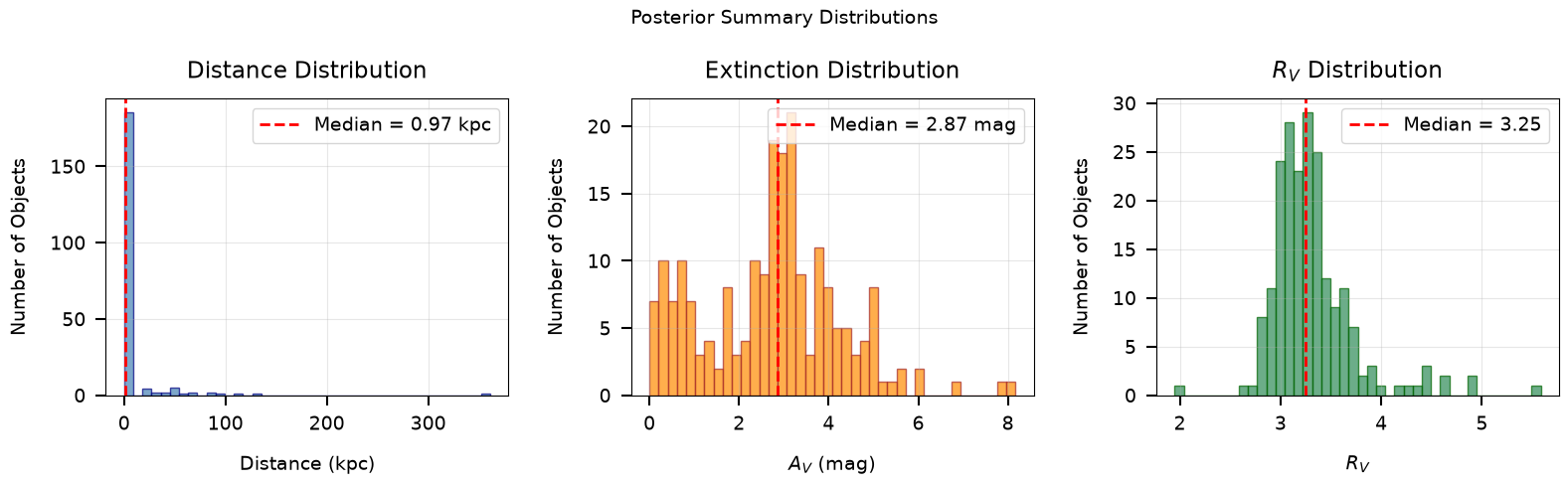
We demonstrate both approaches below and compute medians and 68% credible intervals (16th–84th percentile) using brutus.utils.quantile.

from brutus.utils import quantile

print_section("Section 3: Posterior Summaries")

if not DATA_AVAILABLE:
    print("SKIPPED -- results file not available.")
else:
    q_levels = np.array([0.16, 0.50, 0.84])

    # --- Approach 1: Use pre-computed samps_dist / samps_red / samps_dred ---
    samps_dist = results["samps_dist"]   # kpc
    samps_red = results["samps_red"]     # A_V
    samps_dred = results["samps_dred"]   # R_V

    Nobj = samps_dist.shape[0]

    # Storage for summaries
    dist_lo = np.full(Nobj, np.nan)
    dist_med = np.full(Nobj, np.nan)
    dist_hi = np.full(Nobj, np.nan)
    av_lo = np.full(Nobj, np.nan)
    av_med = np.full(Nobj, np.nan)
    av_hi = np.full(Nobj, np.nan)
    rv_lo = np.full(Nobj, np.nan)
    rv_med = np.full(Nobj, np.nan)
    rv_hi = np.full(Nobj, np.nan)

    for i in range(Nobj):
        # Distance (already in kpc)
        d_i = samps_dist[i]
        good = np.isfinite(d_i) & (d_i > 0)
        if np.sum(good) > 1:
            q = quantile(d_i[good], q_levels)
            dist_lo[i], dist_med[i], dist_hi[i] = q

        # A_V
        av_i = samps_red[i]
        good_av = np.isfinite(av_i)
        if np.sum(good_av) > 1:
            q = quantile(av_i[good_av], q_levels)
            av_lo[i], av_med[i], av_hi[i] = q

        # R_V
        rv_i = samps_dred[i]
        good_rv = np.isfinite(rv_i)
        if np.sum(good_rv) > 1:
            q = quantile(rv_i[good_rv], q_levels)
            rv_lo[i], rv_med[i], rv_hi[i] = q

    # Print a table for the first 10 objects
    n_show = min(10, Nobj)
    print("Using pre-computed samps_dist / samps_red / samps_dred:\n")
    print(f"{'Obj':>5s}  {'d_med (kpc)':>12s}  {'d_lo':>8s}  {'d_hi':>8s}  "
          f"{'AV_med':>8s}  {'AV_lo':>8s}  {'AV_hi':>8s}  "
          f"{'RV_med':>8s}")
    print(f"{'---':>5s}  {'----------':>12s}  {'----':>8s}  {'----':>8s}  "
          f"{'------':>8s}  {'-----':>8s}  {'-----':>8s}  "
          f"{'------':>8s}")
    for i in range(n_show):
        print(
            f"{i:5d}  {dist_med[i]:12.3f}  {dist_lo[i]:8.3f}  {dist_hi[i]:8.3f}  "
            f"{av_med[i]:8.3f}  {av_lo[i]:8.3f}  {av_hi[i]:8.3f}  "
            f"{rv_med[i]:8.3f}"
        )

    print(f"\n... ({Nobj} objects total)")

    # Global summary
    valid_d = np.isfinite(dist_med)
    print(f"\nGlobal distance summary ({np.sum(valid_d)} valid objects):")
    print(f"  Median distance: {np.nanmedian(dist_med):.3f} kpc")
    print(f"  Range: [{np.nanmin(dist_med):.3f}, {np.nanmax(dist_med):.3f}] kpc")

    # --- Approach 2: Convert ml_scale manually (for reference) ---
    # Scale factor: s = 1/d_kpc^2, so d_kpc = 1/sqrt(s)
    print("\n--- Manual conversion from ml_scale (for reference) ---")
    scales = results["ml_scale"]
    s_med = np.nanmedian(scales, axis=1)
    good_s = np.isfinite(s_med) & (s_med > 0)
    d_from_scale = np.full(Nobj, np.nan)
    d_from_scale[good_s] = 1.0 / np.sqrt(s_med[good_s])  # kpc
    print(f"  Median distance from ml_scale: {np.nanmedian(d_from_scale):.3f} kpc")
    print(f"  (cf. samps_dist median: {np.nanmedian(dist_med):.3f} kpc)")
    print("  These differ because samps_dist incorporates the distance and"
          "  parallax priors applied during the fit's MC integration.")

Section 3: Posterior Summaries
==============================
Using pre-computed samps_dist / samps_red / samps_dred:

  Obj   d_med (kpc)      d_lo      d_hi    AV_med     AV_lo     AV_hi    RV_med
  ---    ----------      ----      ----    ------     -----     -----    ------
    0         0.284     0.279     0.291     0.203     0.049     0.533     3.406
    1         1.213     1.159     1.296     5.058     4.982     5.140     2.804
    2         0.972     0.882     1.106     5.495     5.385     5.655     2.938
    3         0.364     0.358     0.370     1.686     0.131     1.900     3.360
    4         1.001     0.892     1.143     5.215     4.964     5.351     2.924
    5         0.340     0.337     0.343     2.846     2.806     2.912     3.640
    6        65.620    43.593    78.102     1.074     0.972     1.332     3.235
    7         0.854     0.843     0.880     4.034     3.832     4.309     3.043
    8         0.483     0.448     0.515     4.988     4.746     5.239     2.860
    9         1.144     1.019     1.185     2.775     2.587     3.089     3.214

... (207 objects total)

Global distance summary (207 valid objects):
  Median distance: 0.972 kpc
  Range: [0.069, 361.095] kpc

--- Manual conversion from ml_scale (for reference) ---
  Median distance from ml_scale: 0.968 kpc
  (cf. samps_dist median: 0.972 kpc)
  These differ because samps_dist incorporates the distance and  parallax priors applied during the fit's MC integration.

# Plot a distance histogram
if DATA_AVAILABLE:
    fig, axes = plt.subplots(1, 3, figsize=(16, 5))

    # Panel 1: Distance distribution
    ax = axes[0]
    valid_d = dist_med[np.isfinite(dist_med)]
    ax.hist(valid_d, bins=40, alpha=0.7, color="steelblue", edgecolor="navy")
    ax.axvline(
        np.median(valid_d), color="red", ls="--", lw=2,
        label=f"Median = {np.median(valid_d):.2f} kpc"
    )
    ax.set_xlabel("Distance (kpc)")
    ax.set_ylabel("Number of Objects")
    ax.set_title("Distance Distribution")
    ax.legend()
    ax.grid(True, alpha=0.3)

    # Panel 2: A_V distribution
    ax = axes[1]
    valid_av = av_med[np.isfinite(av_med)]
    ax.hist(valid_av, bins=40, alpha=0.7, color="darkorange", edgecolor="brown")
    ax.axvline(
        np.median(valid_av), color="red", ls="--", lw=2,
        label=f"Median = {np.median(valid_av):.2f} mag"
    )
    ax.set_xlabel(r"$A_V$ (mag)")
    ax.set_ylabel("Number of Objects")
    ax.set_title("Extinction Distribution")
    ax.legend()
    ax.grid(True, alpha=0.3)

    # Panel 3: R_V distribution
    ax = axes[2]
    valid_rv = rv_med[np.isfinite(rv_med)]
    ax.hist(valid_rv, bins=40, alpha=0.7, color="seagreen", edgecolor="darkgreen")
    ax.axvline(
        np.median(valid_rv), color="red", ls="--", lw=2,
        label=f"Median = {np.median(valid_rv):.2f}"
    )
    ax.set_xlabel(r"$R_V$")
    ax.set_ylabel("Number of Objects")
    ax.set_title(r"$R_V$ Distribution")
    ax.legend()
    ax.grid(True, alpha=0.3)

    plt.suptitle("Posterior Summary Distributions", fontsize=14)
    save_figure(fig, 11, "posterior_summaries")
    plt.show()

    print("Histograms of median posterior values for all objects.")
else:
    print("SKIPPED -- results file not available.")

  Saved: /home/user/brutus/tutorials/plots/tutorial_11/posterior_summaries.png

../_images/bc9462a8579c0e7ab600d3b2872affd33b56406a1c4f6a8fe35a974803808448.png

Histograms of median posterior values for all objects.

Section 4: Sampling from Posteriors#

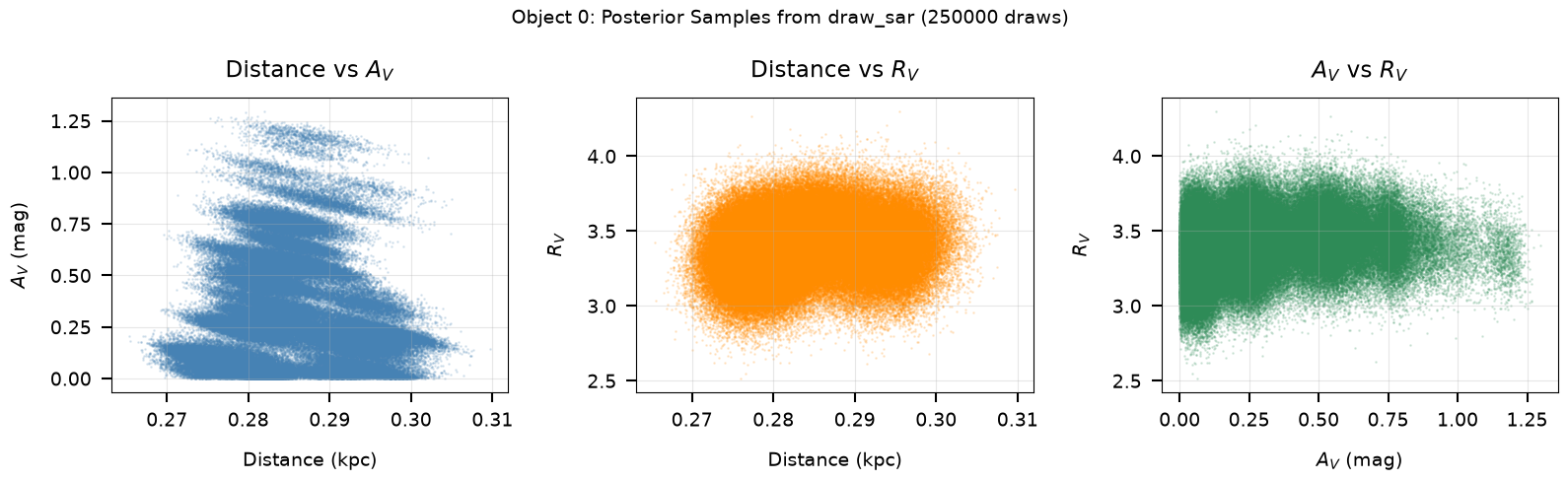
The draw_sar function generates Monte Carlo draws from the joint (s, A_V, R_V) posterior for a single object. It uses the per-sample ML estimates (ml_scale, ml_av, ml_rv) and local covariance matrices ml_cov_sar, drawing from multivariate normals and rejection-sampling to enforce physical bounds on A_V and R_V.

This is the standard way to generate posterior realizations for downstream analysis (e.g., propagating uncertainties into derived quantities like absolute magnitude or bolometric luminosity).

Function signature#

draw_sar(scales, avs, rvs, covs_sar, ndraws=500,
         avlim=(0., 6.), rvlim=(1., 8.), rstate=None,
         max_attempts=10000)

Returns (sdraws, adraws, rdraws) each of shape (Nsamps, ndraws). Convert scale draws to distance via d_kpc = 1/sqrt(s).

Note: all Nsamps distributions are drawn in a single batched call per rejection pass. The accepted draws follow the same truncated Gaussian distribution as in older brutus versions, but the underlying RNG stream differs, so individual draws are not reproducible against older versions even with a fixed seed. If a distribution has not accumulated ndraws in-bounds samples after max_attempts rejection passes, the remaining slots are padded with the mean values (with a warning).

from brutus.utils import draw_sar

print_section("Section 4: Sampling from Posteriors")

if not DATA_AVAILABLE:
    print("SKIPPED -- results file not available.")
else:
    # Pick one example object
    obj_idx = 0

    scales_obj = results["ml_scale"][obj_idx]
    avs_obj = results["ml_av"][obj_idx]
    rvs_obj = results["ml_rv"][obj_idx]
    covs_obj = results["ml_cov_sar"][obj_idx]

    print(f"Object {obj_idx}:")
    print(f"  ml_scale shape : {scales_obj.shape}")
    print(f"  ml_av shape    : {avs_obj.shape}")
    print(f"  ml_rv shape    : {rvs_obj.shape}")
    print(f"  ml_cov_sar shape: {covs_obj.shape}")

    # Draw 500 (s, A_V, R_V) realizations per sample
    ndraws = 500
    sdraws, adraws, rdraws = draw_sar(
        scales_obj, avs_obj, rvs_obj, covs_obj, ndraws=ndraws
    )

    print(f"\nDraw shapes:")
    print(f"  sdraws: {sdraws.shape}")
    print(f"  adraws: {adraws.shape}")
    print(f"  rdraws: {rdraws.shape}")

    # Flatten draws across all per-model samples
    s_flat = sdraws.ravel()
    a_flat = adraws.ravel()
    r_flat = rdraws.ravel()

    # Convert scale to distance: s = 1/d_kpc^2, so d_kpc = 1/sqrt(s)
    good = np.isfinite(s_flat) & (s_flat > 0)
    d_flat = np.full_like(s_flat, np.nan)
    d_flat[good] = 1.0 / np.sqrt(s_flat[good])  # kpc

    print(f"\nTotal draws (flattened): {len(s_flat)}")
    print(f"  Distance: median = {np.nanmedian(d_flat):.3f} kpc")
    print(f"  A_V     : median = {np.nanmedian(a_flat):.3f} mag")
    print(f"  R_V     : median = {np.nanmedian(r_flat):.3f}")

    # Compare with pre-computed samps_dist
    print(f"\nComparison with pre-computed samps_dist:")
    print(f"  samps_dist median: {np.nanmedian(results['samps_dist'][obj_idx]):.3f} kpc")
    print(f"  draw_sar median  : {np.nanmedian(d_flat):.3f} kpc")

Section 4: Sampling from Posteriors
===================================
Object 0:
  ml_scale shape : (500,)
  ml_av shape    : (500,)
  ml_rv shape    : (500,)
  ml_cov_sar shape: (500, 3, 3)

Draw shapes:
  sdraws: (500, 500)
  adraws: (500, 500)
  rdraws: (500, 500)

Total draws (flattened): 250000
  Distance: median = 0.282 kpc
  A_V     : median = 0.198 mag
  R_V     : median = 3.392

Comparison with pre-computed samps_dist:
  samps_dist median: 0.284 kpc
  draw_sar median  : 0.282 kpc

# Corner-like scatter plot of the drawn posterior samples
if DATA_AVAILABLE:
    fig, axes = plt.subplots(1, 3, figsize=(16, 5))

    # Use only finite draws
    mask_good = np.isfinite(d_flat) & np.isfinite(a_flat) & np.isfinite(r_flat)
    d_plot = d_flat[mask_good]
    a_plot = a_flat[mask_good]
    r_plot = r_flat[mask_good]

    # Panel 1: Distance vs A_V
    ax = axes[0]
    ax.scatter(d_plot, a_plot, s=1, alpha=0.15, color="steelblue")
    ax.set_xlabel("Distance (kpc)")
    ax.set_ylabel(r"$A_V$ (mag)")
    ax.set_title(r"Distance vs $A_V$")
    ax.grid(True, alpha=0.3)

    # Panel 2: Distance vs R_V
    ax = axes[1]
    ax.scatter(d_plot, r_plot, s=1, alpha=0.15, color="darkorange")
    ax.set_xlabel("Distance (kpc)")
    ax.set_ylabel(r"$R_V$")
    ax.set_title(r"Distance vs $R_V$")
    ax.grid(True, alpha=0.3)

    # Panel 3: A_V vs R_V
    ax = axes[2]
    ax.scatter(a_plot, r_plot, s=1, alpha=0.15, color="seagreen")
    ax.set_xlabel(r"$A_V$ (mag)")
    ax.set_ylabel(r"$R_V$")
    ax.set_title(r"$A_V$ vs $R_V$")
    ax.grid(True, alpha=0.3)

    plt.suptitle(
        f"Object {obj_idx}: Posterior Samples from draw_sar "
        f"({len(d_plot)} draws)",
        fontsize=14,
    )
    save_figure(fig, 11, "draw_sar_scatter")
    plt.show()

    print("Corner-like scatter of (distance, A_V, R_V) posterior draws.")
    print("Correlations between parameters are visible in the scatter patterns.")
else:
    print("SKIPPED -- results file not available.")

  Saved: /home/user/brutus/tutorials/plots/tutorial_11/draw_sar_scatter.png

../_images/838e1931f6cae14cffd88ce4c3f4adc980e8abe7fa39722e799d1371d6c457ac.png

Corner-like scatter of (distance, A_V, R_V) posterior draws.
Correlations between parameters are visible in the scatter patterns.

Section 5: Photometric Conversions#

BruteForce works internally with linear flux densities (maggies), not magnitudes. The utility functions magnitude and inv_magnitude convert between the two representations:

$$\mathrm{flux} = 10^{-0.4 \times \mathrm{mag}}, \qquad \mathrm{mag} = -2.5 \log_{10}(\mathrm{flux})$$

This section demonstrates the round-trip conversion and, if the input photometry file is available, shows a comparison between the two representations.

from brutus.utils import magnitude, inv_magnitude

print_section("Section 5: Photometric Conversions")

# Demonstrate round-trip on synthetic data
np.random.seed(42)
mag_synth = np.random.uniform(14, 22, size=(5, 4))
magerr_synth = np.random.uniform(0.01, 0.1, size=(5, 4))

flux_synth, fluxerr_synth = inv_magnitude(mag_synth, magerr_synth)
mag_recov, magerr_recov = magnitude(flux_synth, fluxerr_synth)

residual = np.max(np.abs(mag_synth - mag_recov))
print(f"Round-trip mag -> flux -> mag:")
print(f"  Max |mag residual| = {residual:.2e}")
assert np.allclose(mag_synth, mag_recov, atol=1e-12), "Round-trip failed"
print("  Round-trip verified: exact to machine precision.")

# Load input photometry if available
PHOT_AVAILABLE = False
try:
    import h5py

    phot_path = find_brutus_data_file("Orion_l209.1_b-19.9.h5")
    with h5py.File(phot_path, "r") as f:
        fpix = f["photometry"]["pixel 0-0"]
        input_mag = fpix["mag"][:]
        input_magerr = fpix["err"][:]
        input_flux, input_fluxerr = inv_magnitude(input_mag, input_magerr)
        input_mask = np.isfinite(input_magerr)

    PHOT_AVAILABLE = True
    print(f"\nLoaded input photometry from {phot_path}")
    print(f"  Objects: {input_flux.shape[0]}, Filters: {input_flux.shape[1]}")
    print(f"  Example (object 0):")
    print(f"    Magnitudes: {input_mag[0]}")
    print(f"    Fluxes    : {input_flux[0]}")
except (FileNotFoundError, ImportError) as exc:
    print(f"\nInput photometry file not found (optional).")
    print(f"  ({exc})")

Section 5: Photometric Conversions
==================================
Round-trip mag -> flux -> mag:
  Max |mag residual| = 3.55e-15
  Round-trip verified: exact to machine precision.

Loaded input photometry from /home/user/brutus/tutorials/Orion_l209.1_b-19.9.h5
  Objects: 207, Filters: 8
  Example (object 0):
    Magnitudes: [16.922836 15.631483 14.976083 14.652597 14.47464  13.423    12.693
 12.522   ]
    Fluxes    : [1.7016313e-07 5.5899312e-07 1.0222727e-06 1.3770853e-06 1.6223481e-06
 4.2736583e-06 8.3714385e-06 9.7994107e-06]

Section 6: Visualization#

The brutus.plotting module provides two key functions for visualizing BruteForce results:

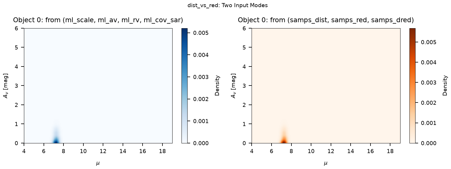
dist_vs_red: 2-D density plot of the joint distance-reddening posterior. We use it here for a single object; multi-object input (arrays of shape (Nobj, Nsamps)) is also accepted, in which case the average of the per-object 2-D PDFs is plotted.
cornerplot: Full corner plot of all stellar parameters plus (A_V, R_V, distance). Requires the model grid in memory.

Below we demonstrate dist_vs_red (which only needs the results file) and note the requirements for cornerplot.

from brutus.plotting import dist_vs_red

print_section("Section 6: dist_vs_red Visualization")

if not DATA_AVAILABLE:
    print("SKIPPED -- results file not available.")
else:
    obj_idx = 0

    # dist_vs_red accepts either a 4-tuple (scales, avs, rvs, covs_sar)
    # or a 3-tuple (dists, reds, dreds) of pre-computed samples.
    # Here we demonstrate both approaches.

    # Approach 1: 4-tuple with ML estimates and covariances
    # (dist_vs_red will call draw_sar internally)
    data_tuple_4 = (
        results["ml_scale"][obj_idx],
        results["ml_av"][obj_idx],
        results["ml_rv"][obj_idx],
        results["ml_cov_sar"][obj_idx],
    )

    # Approach 2: 3-tuple with pre-computed distance/reddening draws
    data_tuple_3 = (
        results["samps_dist"][obj_idx],
        results["samps_red"][obj_idx],
        results["samps_dred"][obj_idx],
    )

    # Use the Orion field centre as a default coordinate
    coord = (209.1, -19.9)

    fig, axes = plt.subplots(1, 2, figsize=(16, 6))

    # Panel 1: 4-tuple (ML + covariance -> internal draw_sar)
    plt.sca(axes[0])
    try:
        H1, xe1, ye1, img1 = dist_vs_red(
            data_tuple_4,
            coord=coord,
            dist_type="distance_modulus",
            cmap="Blues",
            smooth=0.015,
            bins=300,
        )
        axes[0].set_title(f"Object {obj_idx}: from (ml_scale, ml_av, ml_rv, ml_cov_sar)")
        plt.colorbar(img1, ax=axes[0], label="Density")
    except Exception as exc:
        axes[0].text(0.5, 0.5, f"Error: {exc}", ha="center", va="center",
                     transform=axes[0].transAxes, fontsize=9)
        axes[0].set_title("4-tuple approach (failed)")

    # Panel 2: 3-tuple (pre-computed samples)
    plt.sca(axes[1])
    try:
        H2, xe2, ye2, img2 = dist_vs_red(
            data_tuple_3,
            coord=coord,
            dist_type="distance_modulus",
            cmap="Oranges",
            smooth=0.015,
            bins=300,
        )
        axes[1].set_title(f"Object {obj_idx}: from (samps_dist, samps_red, samps_dred)")
        plt.colorbar(img2, ax=axes[1], label="Density")
    except Exception as exc:
        axes[1].text(0.5, 0.5, f"Error: {exc}", ha="center", va="center",
                     transform=axes[1].transAxes, fontsize=9)
        axes[1].set_title("3-tuple approach (failed)")

    plt.suptitle("dist_vs_red: Two Input Modes", fontsize=14)
    save_figure(fig, 11, "dist_vs_red_demo")
    plt.show()

    print("Left: 4-tuple input (ml_scale, ml_av, ml_rv, ml_cov_sar).")
    print("Right: 3-tuple input (samps_dist, samps_red, samps_dred).")
    print("Both produce the same distance-reddening posterior density.")

Section 6: dist_vs_red Visualization
====================================

  Saved: /home/user/brutus/tutorials/plots/tutorial_11/dist_vs_red_demo.png

../_images/a4920e8eb965dab060d4bdfe56975446c23754d6b774e5596b68549a3e3b9084.png

Left: 4-tuple input (ml_scale, ml_av, ml_rv, ml_cov_sar).
Right: 3-tuple input (samps_dist, samps_red, samps_dred).
Both produce the same distance-reddening posterior density.

from brutus.plotting import cornerplot

print_section("Section 6b: cornerplot (reference)")

print("cornerplot requires the model grid labels array (from grid_mist_v9.h5)")
print("in addition to the results file. If you have the grid loaded, the call")
print("looks like this:")
print()
print("  fig, axes = cornerplot(")
print("      results['model_idx'][idx],")
print("      (results['ml_scale'][idx], results['ml_av'][idx],")
print("       results['ml_rv'][idx], results['ml_cov_sar'][idx]),")
print("      grid_labels,              # from load_models()")
print("      coord=(l, b),")
print("      parallax=plx,")
print("      parallax_err=plx_err,")
print("      show_titles=True,")
print("  )")
print()
print("See Tutorial 10 (Plotting Functions) for a full worked example.")

Section 6b: cornerplot (reference)
==================================
cornerplot requires the model grid labels array (from grid_mist_v9.h5)
in addition to the results file. If you have the grid loaded, the call
looks like this:

  fig, axes = cornerplot(
      results['model_idx'][idx],
      (results['ml_scale'][idx], results['ml_av'][idx],
       results['ml_rv'][idx], results['ml_cov_sar'][idx]),
      grid_labels,              # from load_models()
      coord=(l, b),
      parallax=plx,
      parallax_err=plx_err,
      show_titles=True,
  )

See Tutorial 10 (Plotting Functions) for a full worked example.

Section 7: Quality Assessment#

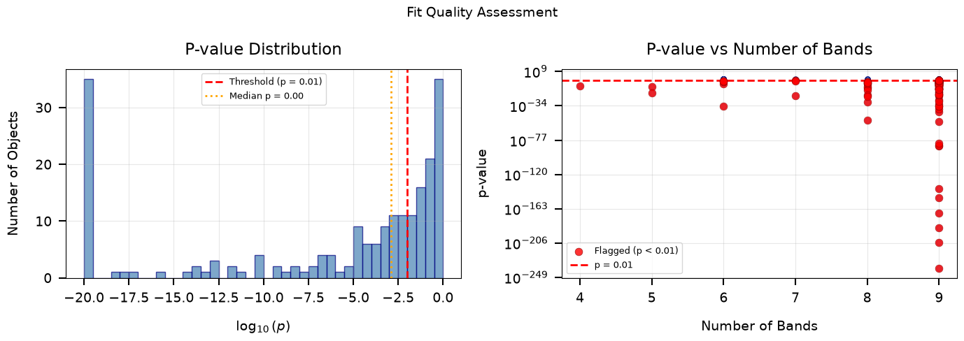
The primary diagnostic for BruteForce results is the p-value derived from the chi-squared distribution. Given the best-fit obj_chi2min and the degrees of freedom dof = Nbands - 3 (three analytically marginalized parameters: s, A_V, R_V), we compute:

$$p = 1 - F_{\chi^2}(\chi^2_{\min};, \mathrm{dof})$$

where $F_{\chi^2}$ is the chi-squared CDF. Small p-values indicate that the observed chi-squared is improbably large under the model, flagging objects that are poorly fit (e.g., binaries, galaxies, problematic photometry).

Why not reduced chi-squared?#

While the reduced chi-squared $\chi^2_\nu = \chi^2/\mathrm{dof}$ is convenient for quick visual checks, it is not variance-stabilizing: its sampling variance is $2/\mathrm{dof}$. This means a fixed threshold like “$\chi^2_\nu > 3$” is far too lenient for objects with many bands (where $\chi^2_\nu$ concentrates tightly around 1) and overly strict for objects with few bands (where the distribution is broad). The p-value approach gives a uniform false-positive rate regardless of the number of bands, making it the principled choice for quality cuts.

Log-evidence#

The output also includes obj_log_evid, an approximate log-evidence (marginal likelihood) computed from the grid-based Laplace approximation. This quantity is most useful for relative model comparison — e.g., comparing how well a MIST grid fits a given star versus an alternative stellar model grid. Its absolute value is not straightforwardly interpretable, so we do not use it as a standalone quality metric here.

from scipy.stats import chi2 as chi2_dist

print_section("Section 7: Quality Assessment")

if not DATA_AVAILABLE:
    print("SKIPPED -- results file not available.")
else:
    chi2 = results["obj_chi2min"]
    Nbands = results["obj_Nbands"]

    # Degrees of freedom: 3 free parameters (s, A_V, R_V)
    n_free = 3
    dof = Nbands - n_free

    # Flag objects with insufficient bands
    insufficient = dof <= 0
    valid = ~insufficient & np.isfinite(chi2)

    print(f"Total objects          : {len(chi2)}")
    print(f"Objects with dof > 0   : {np.sum(~insufficient)}")
    print(f"Objects with dof <= 0  : {np.sum(insufficient)} (too few bands)")

    # Compute p-values from the chi-squared survival function
    pvalues = np.full(len(chi2), np.nan)
    pvalues[valid] = chi2_dist.sf(chi2[valid], dof[valid])

    if np.sum(valid) > 0:
        print(f"\nP-value summary (from chi2 CDF):")
        print(f"  Min     : {np.nanmin(pvalues[valid]):.2e}")
        print(f"  Median  : {np.nanmedian(pvalues[valid]):.3f}")
        print(f"  Max     : {np.nanmax(pvalues[valid]):.3f}")

        # Outlier flagging via p-value threshold
        p_thresh = 0.01
        outliers = valid & (pvalues < p_thresh)
        n_outliers = np.sum(outliers)
        pct_outliers = 100.0 * n_outliers / np.sum(valid)

        print(f"\nOutlier flagging (p < {p_thresh}):")
        print(f"  Flagged : {n_outliers} / {np.sum(valid)} ({pct_outliers:.1f}%)")

        good_fits = valid & (pvalues >= p_thresh)
        print(f"  Good fits: {np.sum(good_fits)} ({100.0 * np.sum(good_fits) / np.sum(valid):.1f}%)")

        # Show the flagged objects
        if n_outliers > 0:
            flagged_idx = np.where(outliers)[0]
            print(f"\n  Flagged objects:")
            print(f"  {'Obj':>5s}  {'chi2':>8s}  {'Nbands':>6s}  {'dof':>4s}  {'chi2/dof':>9s}  {'p-value':>10s}")
            for idx in flagged_idx:
                print(f"  {idx:5d}  {chi2[idx]:8.2f}  {Nbands[idx]:6d}  {dof[idx]:4d}  "
                      f"{chi2[idx]/dof[idx]:9.2f}  {pvalues[idx]:10.2e}")

        # For comparison: show why reduced chi2 thresholds are unreliable
        chi2_dof = chi2[valid] / dof[valid].astype(float)
        print(f"\nFor reference, reduced chi2 (chi2/dof) statistics:")
        print(f"  Median  : {np.median(chi2_dof):.3f}")
        print(f"  Note: The variance of chi2/dof is 2/dof, so a fixed")
        print(f"  threshold means different things at different Nbands.")

    # Log-evidence summary
    print(f"\nLog-evidence (obj_log_evid) summary:")
    lnz = results["obj_log_evid"]
    finite_lnz = lnz[np.isfinite(lnz)]
    if len(finite_lnz) > 0:
        print(f"  Min   : {np.min(finite_lnz):.2f}")
        print(f"  Median: {np.median(finite_lnz):.2f}")
        print(f"  Max   : {np.max(finite_lnz):.2f}")
        print(f"  Note: Useful for relative model comparison (e.g., MIST vs")
        print(f"  alternative grids), not as a standalone quality metric.")
    else:
        print("  (all non-finite)")

Section 7: Quality Assessment
=============================
Total objects          : 207
Objects with dof > 0   : 207
Objects with dof <= 0  : 0 (too few bands)

P-value summary (from chi2 CDF):
  Min     : 0.00e+00
  Median  : 0.001
  Max     : 0.999

Outlier flagging (p < 0.01):
  Flagged : 124 / 207 (59.9%)
  Good fits: 83 (40.1%)

  Flagged objects:
    Obj      chi2  Nbands   dof   chi2/dof     p-value
   50.52       9     6       8.42    3.70e-09
   43.95       9     6       7.33    7.55e-08
   44.65       9     6       7.44    5.48e-08
   60.21       9     6      10.04    4.07e-11
   51.42       9     6       8.57    2.44e-09
   30.75       9     6       5.13    2.82e-05
   25.23       9     6       4.21    3.09e-04
   48.33       9     6       8.06    1.01e-08
   99.24       9     6      16.54    3.62e-19
  140.20       9     6      23.37    9.12e-28
   86.11       9     6      14.35    1.95e-16
   39.28       9     6       6.55    6.30e-07
   62.82       8     5      12.56    3.18e-12
   55.63       8     5      11.13    9.70e-11
   47.34       5     2      23.67    5.26e-11
   43.34       9     6       7.22    1.00e-07
   34.56       8     5       6.91    1.84e-06
  267.10       9     6      44.52    9.07e-55
  210.02       9     6      35.00    1.39e-42
  192.64       9     6      32.11    6.97e-39
  113.27       9     6      18.88    4.21e-22
   74.91       8     5      14.98    9.72e-15
   24.81       9     6       4.13    3.71e-04
   18.90       9     6       3.15    4.33e-03
   93.79       9     6      15.63    4.94e-18
   41.58       9     6       6.93    2.22e-07
   72.37       9     6      12.06    1.34e-13
   42.72       9     6       7.12    1.33e-07
   75.97       9     6      12.66    2.42e-14
   17.83       9     6       2.97    6.68e-03
   54.32       9     6       9.05    6.37e-10
   21.03       9     6       3.50    1.82e-03
   24.95       9     6       4.16    3.48e-04
   27.48       9     6       4.58    1.18e-04
   21.85       9     6       3.64    1.29e-03
   67.44       9     6      11.24    1.37e-12
   23.04       9     6       3.84    7.83e-04
  406.98       9     6      67.83    8.83e-85
 3145.96       9     6     524.33    0.00e+00
 1537.74       9     6     256.29    0.00e+00
 1473.78       9     6     245.63    0.00e+00
  884.18       9     6     147.36   9.86e-188
  708.89       9     6     118.15   7.36e-150
   66.80       9     6      11.13    1.85e-12
 1808.88       9     6     301.48    0.00e+00
  176.85       9     6      29.47    1.59e-35
   26.17       9     6       4.36    2.07e-04
   72.21       9     6      12.03    1.44e-13
  797.35       9     6     132.89   5.74e-169
 1553.39       8     5     310.68    0.00e+00
   20.57       9     6       3.43    2.19e-03
   40.50       9     6       6.75    3.64e-07
  148.44       8     5      29.69    2.87e-30
 1751.24       9     6     291.87    0.00e+00
   25.82       8     5       5.16    9.66e-05
   14.96       7     4       3.74    4.77e-03
   37.51       4     1      37.51    9.11e-10
  968.95       9     6     161.49   4.64e-206
  657.61       9     6     109.60   8.65e-139
  106.78       8     5      21.36    1.96e-21
   30.53       9     6       5.09    3.11e-05
  252.77       8     5      50.55    1.40e-52
  161.68       9     6      26.95    2.61e-32
   29.25       9     6       4.87    5.46e-05
  405.73       9     6      67.62    1.64e-84
  164.97       6     3      54.99    1.55e-35
   16.85       9     6       2.81    9.84e-03
  106.09       9     6      17.68    1.34e-20
   71.55       9     6      11.92    1.97e-13
   29.98       9     6       5.00    3.96e-05
   28.18       9     6       4.70    8.71e-05
   17.14       9     6       2.86    8.79e-03
  392.73       9     6      65.46    1.02e-81
   17.24       9     6       2.87    8.42e-03
 1118.16       9     6     186.36   2.46e-238
   17.09       7     4       4.27    1.85e-03
   34.37       6     3      11.46    1.65e-07
 3018.65       9     6     503.11    0.00e+00
   82.15       5     2      41.08    1.45e-18
   24.67       9     6       4.11    3.93e-04
   32.95       9     6       5.49    1.07e-05
   29.90       9     6       4.98    4.11e-05
  107.26       7     4      26.81    2.79e-22
   27.91       9     6       4.65    9.78e-05
 1895.54       9     6     315.92    0.00e+00
   24.51       9     6       4.08    4.22e-04
   23.27       9     6       3.88    7.11e-04
   32.29       9     6       5.38    1.43e-05
   34.54       9     6       5.76    5.29e-06
  174.10       9     6      29.02    6.07e-35
   16.97       9     6       2.83    9.41e-03
   26.48       9     6       4.41    1.81e-04
   32.93       9     6       5.49    1.08e-05
   17.90       9     6       2.98    6.49e-03
   74.66       9     6      12.44    4.51e-14
   24.04       9     6       4.01    5.14e-04
  148.15       9     6      24.69    1.90e-29
   32.35       9     6       5.39    1.40e-05
   34.50       9     6       5.75    5.37e-06
   37.97       8     5       7.59    3.83e-07
   48.67       9     6       8.11    8.68e-09
   18.83       9     6       3.14    4.46e-03
   32.92       9     6       5.49    1.09e-05
   21.97       9     6       3.66    1.23e-03
  109.94       9     6      18.32    2.10e-21
   21.55       9     6       3.59    1.46e-03
   17.05       9     6       2.84    9.08e-03
   21.84       9     6       3.64    1.29e-03
  105.95       9     6      17.66    1.43e-20
   23.13       9     6       3.86    7.54e-04
   21.17       9     6       3.53    1.71e-03
   28.83       8     5       5.77    2.50e-05
   58.99       9     6       9.83    7.23e-11
   21.99       9     6       3.66    1.22e-03
   25.40       9     6       4.23    2.88e-04
   16.45       6     3       5.48    9.17e-04
   39.67       9     6       6.61    5.29e-07
   19.48       6     3       6.49    2.17e-04
   30.77       8     5       6.15    1.04e-05
   76.26       9     6      12.71    2.11e-14
   20.88       9     6       3.48    1.93e-03
  114.76       8     5      22.95    4.04e-23
   15.57       6     3       5.19    1.39e-03
   19.34       9     6       3.22    3.63e-03

For reference, reduced chi2 (chi2/dof) statistics:
  Median  : 3.840
  Note: The variance of chi2/dof is 2/dof, so a fixed
  threshold means different things at different Nbands.

Log-evidence (obj_log_evid) summary:
  Min   : -15847.17
  Median: 83.74
  Max   : 124.41
  Note: Useful for relative model comparison (e.g., MIST vs
  alternative grids), not as a standalone quality metric.

# P-value quality assessment plots
if DATA_AVAILABLE and np.sum(valid) > 0:
    fig, axes = plt.subplots(1, 2, figsize=(14, 5))

    # Panel 1: P-value histogram (log scale)
    ax = axes[0]
    pvals_plot = pvalues[valid]
    # Use log10(p) for better visualization of the distribution
    log_pvals = np.log10(np.clip(pvals_plot, 1e-20, 1.0))
    ax.hist(
        log_pvals, bins=40, alpha=0.7,
        color="steelblue", edgecolor="navy"
    )
    ax.axvline(
        np.log10(p_thresh), color="red", ls="--", lw=2,
        label=f"Threshold (p = {p_thresh})"
    )
    ax.axvline(
        np.log10(np.median(pvals_plot)), color="orange", ls=":", lw=2,
        label=f"Median p = {np.median(pvals_plot):.2f}"
    )
    ax.set_xlabel(r"$\log_{10}(p)$")
    ax.set_ylabel("Number of Objects")
    ax.set_title("P-value Distribution")
    ax.legend(fontsize=9)
    ax.grid(True, alpha=0.3)

    # Panel 2: P-value vs number of bands
    ax = axes[1]
    ax.scatter(
        Nbands[valid], pvalues[valid],
        s=30, alpha=0.6, color="steelblue", edgecolor="navy", lw=0.5
    )
    # Highlight flagged objects
    if np.sum(outliers) > 0:
        ax.scatter(
            Nbands[outliers], pvalues[outliers],
            s=60, alpha=0.8, color="red", edgecolor="darkred", lw=0.5,
            label=f"Flagged (p < {p_thresh})", zorder=5
        )
    ax.axhline(
        p_thresh, color="red", ls="--", lw=2,
        label=f"p = {p_thresh}"
    )
    ax.set_xlabel("Number of Bands")
    ax.set_ylabel("p-value")
    ax.set_yscale("log")
    ax.set_title("P-value vs Number of Bands")
    ax.legend(fontsize=9)
    ax.grid(True, alpha=0.3)

    plt.suptitle("Fit Quality Assessment", fontsize=14)
    save_figure(fig, 11, "chi2_quality")
    plt.show()

    print("Left: histogram of log10(p-value) from the chi2 CDF.")
    print("Right: p-value vs number of bands. Unlike reduced chi2, the")
    print("p-value threshold gives a uniform false-positive rate across")
    print("all band counts.")
else:
    print("SKIPPED -- results file not available or no valid chi2 values.")

  Saved: /home/user/brutus/tutorials/plots/tutorial_11/chi2_quality.png

../_images/a644ea3c9a8a742053bbc732a856c537ceeeb2146d194c1faf1ea0f7bc70f0d2.png

Left: histogram of log10(p-value) from the chi2 CDF.
Right: p-value vs number of bands. Unlike reduced chi2, the
p-value threshold gives a uniform false-positive rate across
all band counts.

Summary#

This tutorial demonstrated how to work with BruteForce output files:

Key Steps#

Loading – Use load_example_results() or open directly with h5py. Inspect top-level keys, shapes, and dtypes to understand the file layout.
Output arrays – Per-sample arrays (model_idx, ml_scale, ml_av, ml_rv, ml_cov_sar), pre-computed draws (samps_dist, samps_red, samps_dred), and per-object summaries (obj_chi2min, obj_Nbands, obj_log_evid).
Posterior summaries – Use samps_dist / samps_red / samps_dred for ready-to-use posterior samples, or convert ml_scale manually via d_kpc = 1/sqrt(s) where s = 1/d_kpc^2. Compute quantiles with brutus.utils.quantile.
Posterior sampling – draw_sar generates Monte Carlo draws from the joint (s, A_V, R_V) posterior using the stored covariance matrices.
Photometric conversions – magnitude and inv_magnitude convert between flux (maggies) and AB magnitudes.
Visualization – dist_vs_red shows the 2-D distance-reddening posterior (accepts either 4-tuple or 3-tuple input); cornerplot provides a full multi-parameter view (requires the model grid).
Quality assessment – Compute p-values from obj_chi2min via the chi-squared CDF (scipy.stats.chi2.sf). Flag objects with small p-values (e.g., p < 0.01) as poorly fit. Avoid using reduced chi-squared thresholds, which are not variance-stabilizing and behave inconsistently across different numbers of bands. The log-evidence obj_log_evid is useful for relative model comparison but not as a standalone quality metric.