Tutorial 9: Utility Functions

This tutorial provides a hands-on tour of the utility functions in brutus.utils. These functions underpin much of the core analysis in brutus but are also useful on their own for photometric conversions, statistical computations, and posterior sampling.

Topics Covered

1. Photometry conversions – magnitudes, luptitudes, and flux arithmetic

2. Photometric likelihoods – standard and outlier models

3. Mathematical utilities – matrix inversion, positive-definiteness checks, distribution functions

4. Sampling utilities – weighted quantiles, multivariate normal sampling, posterior draws

Prerequisites

This notebook requires no external data files. All demonstrations use synthetic data generated on the fly.

# Setup: imports and plot style
import warnings

import numpy as np
import matplotlib.pyplot as plt

warnings.filterwarnings("ignore")

# Tutorial utilities
from tutorial_utils import (
    setup_tutorial,
    save_figure,
    print_section,
    assert_array_properties,
)

# Run the standardized tutorial bootstrap
info = setup_tutorial(9, title="Tutorial 09: Utility Functions")

# Matplotlib defaults for this notebook
plt.rcParams["figure.figsize"] = (10, 6)

Tutorial 09: Utility Functions
==============================

Checking data requirements for Tutorial 9
=========================================

  All required files available

1. Photometry Conversions

brutus works internally with linear flux densities rather than magnitudes. The brutus.utils module provides functions for converting between the two representations, as well as support for asinh magnitudes (“luptitudes”) that behave better at faint flux levels.

Key functions

Function	Description
magnitude	Flux to AB magnitude
inv_magnitude	AB magnitude to flux
luptitude	Flux to asinh magnitude (Lupton et al. 1999)
inv_luptitude	Asinh magnitude to flux
add_mag	Combine fluxes in magnitude space
Note on units: brutus accepts photometry as linear flux densities
in native survey units – specifically “maggies” (i.e., $10^{-0.4m}$
where $m$ is the magnitude in native survey units). The conversion
functions below (magnitude, inv_magnitude, etc.) handle the
transformation between magnitudes and this linear flux representation.

from brutus.utils import magnitude, inv_magnitude

print_section("1a. Magnitude / Flux Round-Trip")

# Create synthetic magnitude data: 5 objects, 4 filters
np.random.seed(42)
mag_orig = np.random.uniform(14, 22, size=(5, 4))
mag_err_orig = np.random.uniform(0.01, 0.1, size=(5, 4))

print("Original magnitudes (first object):")
print(f"  mag     = {mag_orig[0]}")
print(f"  mag_err = {mag_err_orig[0]}")

# Convert mag -> flux -> mag
flux, flux_err = inv_magnitude(mag_orig, mag_err_orig)
mag_recovered, mag_err_recovered = magnitude(flux, flux_err)

print("\nRecovered magnitudes (first object):")
print(f"  mag     = {mag_recovered[0]}")
print(f"  mag_err = {mag_err_recovered[0]}")

# Verify round-trip
mag_residual = np.max(np.abs(mag_orig - mag_recovered))
err_residual = np.max(np.abs(mag_err_orig - mag_err_recovered))
print(f"\nMax magnitude residual : {mag_residual:.2e}")
print(f"Max error residual    : {err_residual:.2e}")

assert np.allclose(mag_orig, mag_recovered, atol=1e-12), "Magnitude round-trip failed"
assert np.allclose(mag_err_orig, mag_err_recovered, atol=1e-12), "Error round-trip failed"
print("\nRound-trip verified: mag -> flux -> mag is exact.")

1a. Magnitude / Flux Round-Trip
===============================
Original magnitudes (first object):
  mag     = [16.99632095 21.60571445 19.85595153 18.78926787]
  mag_err = [0.06506676 0.02255445 0.03629302 0.04297257]

Recovered magnitudes (first object):
  mag     = [16.99632095 21.60571445 19.85595153 18.78926787]
  mag_err = [0.06506676 0.02255445 0.03629302 0.04297257]

Max magnitude residual : 3.55e-15
Max error residual    : 1.39e-17

Round-trip verified: mag -> flux -> mag is exact.

from brutus.utils import luptitude, inv_luptitude

print_section("1b. Luptitude (Asinh Magnitude) Round-Trip")

# Use the same synthetic flux data from above
skynoise = 1e-9  # softening parameter

# flux -> luptitude -> flux
lupt, lupt_err = luptitude(flux, flux_err, skynoise=skynoise)
flux_recovered, flux_err_recovered = inv_luptitude(lupt, lupt_err, skynoise=skynoise)

print("Original flux (first object):")
print(f"  flux     = {flux[0]}")
print(f"\nRecovered flux (first object):")
print(f"  flux     = {flux_recovered[0]}")

flux_residual = np.max(np.abs(flux - flux_recovered))
print(f"\nMax flux residual: {flux_residual:.2e}")

assert np.allclose(flux, flux_recovered, rtol=1e-10), "Luptitude round-trip failed"
print("Round-trip verified: flux -> luptitude -> flux is exact.")

# Compare magnitude vs luptitude for the same data
mag_from_flux, _ = magnitude(flux, flux_err)
print(f"\nMagnitude vs Luptitude (first object):")
print(f"  mag  = {mag_from_flux[0]}")
print(f"  lupt = {lupt[0]}")
print(f"  diff = {mag_from_flux[0] - lupt[0]}")
print("\nFor bright sources the two systems are nearly identical.")

1b. Luptitude (Asinh Magnitude) Round-Trip
==========================================
Original flux (first object):
  flux     = [1.59027276e-07 2.27884202e-09 1.14187716e-08 3.04995092e-08]

Recovered flux (first object):
  flux     = [1.59027276e-07 2.27884202e-09 1.14187716e-08 3.04995092e-08]

Max flux residual: 2.12e-21
Round-trip verified: flux -> luptitude -> flux is exact.

Magnitude vs Luptitude (first object):
  mag  = [16.99632095 21.60571445 19.85595153 18.78926787]
  lupt = [16.99627802 21.43966326 19.84771879 18.78810257]
  diff = [4.29294498e-05 1.66051189e-01 8.23274868e-03 1.16530448e-03]

For bright sources the two systems are nearly identical.

from brutus.utils import add_mag

print_section("1c. Adding Magnitudes (Combining Fluxes)")

# Two equal-brightness stars: combined flux should be double,
# which is -2.5 * log10(2) ~ -0.75 mag brighter.
mag1 = np.array([15.0, 18.0, 20.0])
mag2 = np.array([15.0, 18.0, 20.0])

mag_combined = add_mag(mag1, mag2)

expected_shift = -2.5 * np.log10(2)
print(f"Two equal stars (mag = {mag1}):")
print(f"  Combined   = {mag_combined}")
print(f"  Expected   = {mag1 + expected_shift}")
print(f"  Shift      = {expected_shift:.4f} mag (= -2.5 * log10(2))")

assert np.allclose(mag_combined, mag1 + expected_shift, atol=1e-12)

# Unequal stars: 5-mag difference means 100x flux ratio
mag_a = np.array([15.0])
mag_b = np.array([20.0])
print(f"\nBright (mag=15) + faint (mag=20):")
print(f"  Combined = {add_mag(mag_a, mag_b)[0]:.4f} (barely changes the bright star)")

1c. Adding Magnitudes (Combining Fluxes)
========================================
Two equal stars (mag = [15. 18. 20.]):
  Combined   = [14.24742501 17.24742501 19.24742501]
  Expected   = [14.24742501 17.24742501 19.24742501]
  Shift      = -0.7526 mag (= -2.5 * log10(2))

Bright (mag=15) + faint (mag=20):
  Combined = 14.9892 (barely changes the bright star)

Show code cell source

Hide code cell source

print_section("1d. Magnitude vs Luptitude at Faint Fluxes")

# Demonstrate where luptitudes diverge from magnitudes
flux_range = np.logspace(-12, -4, 500).reshape(1, -1)  # shape (1, N) for API
flux_err_range = 0.1 * flux_range  # 10% errors

skynoise_demo = 1e-9

mag_vals, _ = magnitude(flux_range, flux_err_range)
lupt_vals, _ = luptitude(flux_range, flux_err_range, skynoise=skynoise_demo)

fig, axes = plt.subplots(1, 2, figsize=(14, 5))

# Left: magnitude and luptitude vs flux
ax = axes[0]
ax.plot(flux_range.ravel(), mag_vals.ravel(), "b-", lw=2, label="magnitude")
ax.plot(flux_range.ravel(), lupt_vals.ravel(), "r--", lw=2, label="luptitude")
ax.axvline(skynoise_demo, color="gray", ls=":", lw=1.5, label=f"skynoise = {skynoise_demo:.0e}")
ax.set_xscale("log")
ax.set_xlabel("Flux")
ax.set_ylabel("Magnitude / Luptitude")
ax.set_title("Magnitude vs Luptitude")
ax.legend(loc="upper right")
ax.invert_yaxis()
ax.grid(True, alpha=0.3)

# Right: difference
ax = axes[1]
diff = mag_vals.ravel() - lupt_vals.ravel()
ax.plot(flux_range.ravel(), diff, "k-", lw=2)
ax.axhline(0, color="gray", ls="--", lw=1)
ax.axvline(skynoise_demo, color="gray", ls=":", lw=1.5, label=f"skynoise = {skynoise_demo:.0e}")
ax.set_xscale("log")
ax.set_xlabel("Flux")
ax.set_ylabel("mag - lupt")
ax.set_title("Difference (magnitude minus luptitude)")
ax.legend()
ax.grid(True, alpha=0.3)

plt.suptitle("Luptitudes converge to magnitudes at high flux,\n"
             "but remain well-behaved at low flux", fontsize=13)
save_figure(fig, 9, "mag_vs_luptitude")
plt.show()

print("At bright fluxes the two systems agree to < 0.001 mag.")
print("Near the sky noise level, luptitudes remain finite while magnitudes diverge.")

1d. Magnitude vs Luptitude at Faint Fluxes
==========================================

  Saved: /mnt/c/Users/joshs/Dropbox/GitHub/brutus/tutorials/plots/tutorial_09/mag_vs_luptitude.png

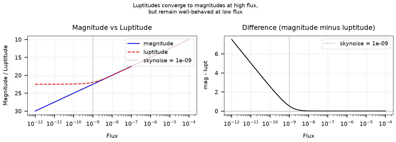
At bright fluxes the two systems agree to < 0.001 mag.
Near the sky noise level, luptitudes remain finite while magnitudes diverge.

2. Photometric Likelihoods

The phot_loglike function computes the log-likelihood of observed photometry given a set of model fluxes. Two additional functions provide outlier models:

Function	Description
phot_loglike	Standard Gaussian photometric log-likelihood
chisquare_outlier_loglike	Chi-square based outlier model (for dim_prior=True)
uniform_outlier_loglike	Quasi-uniform outlier model (for dim_prior=False)

from brutus.utils import phot_loglike
from brutus.utils.photometry import chisquare_outlier_loglike, uniform_outlier_loglike

print_section("2a. Photometric Log-Likelihood")

np.random.seed(123)

# One observed object with 5 filters
Nfilt = 5
true_flux = np.array([[1.0, 2.0, 3.0, 1.5, 0.8]])  # shape (1, 5)
obs_err = np.array([[0.1, 0.15, 0.2, 0.12, 0.08]])  # shape (1, 5)

# Create 100 model fluxes: good match, mediocre, and poor
Nmod = 100
# Models are spread around the truth with varying offsets
offsets = np.linspace(-1.5, 1.5, Nmod)
model_fluxes = true_flux[:, None, :] + offsets[None, :, None] * obs_err[:, None, :]
# shape: (1, 100, 5)

# Compute log-likelihoods
lnl = phot_loglike(true_flux, obs_err, model_fluxes)
lnl_dim = phot_loglike(true_flux, obs_err, model_fluxes, dim_prior=True)

print(f"Observed flux shape   : {true_flux.shape}")
print(f"Model flux shape      : {model_fluxes.shape}")
print(f"Log-likelihood shape  : {lnl.shape}")
print(f"\nBest log-likelihood (no dim_prior) : {lnl.max():.4f}")
print(f"Best log-likelihood (dim_prior)     : {lnl_dim.max():.4f}")

assert_array_properties(lnl, name="lnl", ndim=2, shape=(1, Nmod), finite=True)
print("\nLog-likelihood array properties verified.")

2a. Photometric Log-Likelihood
==============================
Observed flux shape   : (1, 5)
Model flux shape      : (1, 100, 5)
Log-likelihood shape  : (1, 100)

Best log-likelihood (no dim_prior) : 5.8599
Best log-likelihood (dim_prior)     : -1.8696

Log-likelihood array properties verified.

print_section("2b. Outlier Models")

# Compute outlier log-likelihoods for the observed object
lnl_chisq_outlier = chisquare_outlier_loglike(true_flux, obs_err)
lnl_uniform_outlier = uniform_outlier_loglike(true_flux, obs_err)

print(f"Chi-square outlier log-likelihood : {lnl_chisq_outlier[0]:.4f}")
print(f"Uniform outlier log-likelihood    : {lnl_uniform_outlier[0]:.4f}")
print(f"Best normal model log-likelihood  : {lnl.max():.4f}")

print("\nInterpretation:")
print("  If the best model lnl exceeds the outlier lnl, the object is well-fit.")
print("  If outlier lnl is higher, the object may be a contaminant or artifact.")

assert_array_properties(lnl_chisq_outlier, name="chisq_outlier", ndim=1, shape=(1,), finite=True)
assert_array_properties(lnl_uniform_outlier, name="uniform_outlier", ndim=1, shape=(1,), finite=True)
print("\nOutlier log-likelihood properties verified.")

2b. Outlier Models
==================
Chi-square outlier log-likelihood : -12.3016
Uniform outlier log-likelihood    : 0.0000
Best normal model log-likelihood  : 5.8599

Interpretation:
  If the best model lnl exceeds the outlier lnl, the object is well-fit.
  If outlier lnl is higher, the object may be a contaminant or artifact.

Outlier log-likelihood properties verified.

Show code cell source

Hide code cell source

print_section("2c. Likelihood Comparison Plot")

fig, axes = plt.subplots(1, 2, figsize=(14, 5))

# Left: normal vs dim_prior likelihood curves
ax = axes[0]
ax.plot(offsets, lnl.ravel(), "b-", lw=2, label="phot_loglike")
ax.plot(offsets, lnl_dim.ravel(), "r--", lw=2, label="phot_loglike (dim_prior)")
ax.axhline(lnl_chisq_outlier[0], color="green", ls=":", lw=2,
           label=f"chi-sq outlier ({lnl_chisq_outlier[0]:.1f})")
ax.axhline(lnl_uniform_outlier[0], color="orange", ls=":", lw=2,
           label=f"uniform outlier ({lnl_uniform_outlier[0]:.1f})")
ax.set_xlabel(r"Model offset ($\sigma$ units)")
ax.set_ylabel("Log-likelihood")
ax.set_title("Likelihood vs Model Offset")
ax.legend(fontsize=9, loc="lower center")
ax.grid(True, alpha=0.3)

# Right: probability (exp-normalized)
ax = axes[1]
p_normal = np.exp(lnl.ravel() - lnl.max())
p_dim = np.exp(lnl_dim.ravel() - lnl_dim.max())

ax.plot(offsets, p_normal, "b-", lw=2, label="Standard")
ax.plot(offsets, p_dim, "r--", lw=2, label="With dim_prior")
ax.set_xlabel(r"Model offset ($\sigma$ units)")
ax.set_ylabel("Relative probability")
ax.set_title("Normalized Probability")
ax.legend()
ax.grid(True, alpha=0.3)

plt.suptitle("Photometric Likelihood: Standard vs Outlier Models", fontsize=13)
save_figure(fig, 9, "likelihood_comparison")
plt.show()

print("The standard likelihood peaks when model = data (offset = 0).")
print("The dim_prior version additionally penalizes overfitting (too-perfect matches).")

2c. Likelihood Comparison Plot
==============================

  Saved: /mnt/c/Users/joshs/Dropbox/GitHub/brutus/tutorials/plots/tutorial_09/likelihood_comparison.png

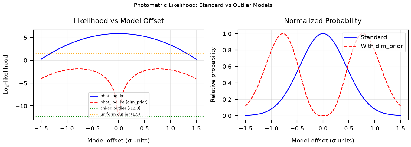
The standard likelihood peaks when model = data (offset = 0).
The dim_prior version additionally penalizes overfitting (too-perfect matches).

3. Mathematical Utilities

The brutus.utils math module provides:

• Fast 3x3 matrix inversion optimized for covariance matrices (inverse3)

• Positive semi-definiteness check (isPSD)

• Chi-square log-PDF (chisquare_logpdf)

• Truncated normal PDF / log-PDF (truncnorm_pdf, truncnorm_logpdf)

from brutus.utils import inverse3, isPSD

print_section("3a. Fast 3x3 Matrix Inversion")

# Create a random positive-definite 3x3 matrix
np.random.seed(99)
L = np.array([[2.0, 0.0, 0.0],
              [0.5, 1.5, 0.0],
              [0.3, 0.2, 1.0]])
A = L @ L.T  # guaranteed positive-definite

print("Matrix A:")
print(A)

# Invert with brutus
A_inv = inverse3(A)

print("\nInverse A_inv:")
print(A_inv)

# Verify: A @ A_inv should be identity
product = A @ A_inv
print("\nA @ A_inv:")
print(product)

identity_error = np.max(np.abs(product - np.eye(3)))
print(f"\nMax deviation from identity: {identity_error:.2e}")

assert np.allclose(product, np.eye(3), atol=1e-10), "Inversion check failed"
print("Verification passed: A @ A_inv = I.")

3a. Fast 3x3 Matrix Inversion
=============================
Matrix A:
[[4.   1.   0.6 ]
 [1.   2.5  0.45]
 [0.6  0.45 1.13]]

Inverse A_inv:
[[ 0.29138889 -0.09555556 -0.11666667]
 [-0.09555556  0.46222222 -0.13333333]
 [-0.11666667 -0.13333333  1.        ]]

A @ A_inv:
[[ 1.00000000e+00 -1.36927506e-17 -8.88178420e-17]
 [ 4.25585493e-18  1.00000000e+00 -6.66133815e-17]
 [-2.42028619e-17 -1.43773882e-17  1.00000000e+00]]

Max deviation from identity: 8.88e-17
Verification passed: A @ A_inv = I.

print_section("3b. Positive Semi-Definiteness Check")

# Test 1: positive-definite matrix (from above)
print(f"A (positive-definite covariance):  isPSD = {isPSD(A)}")

# Test 2: identity matrix
I3 = np.eye(3)
print(f"Identity matrix:                   isPSD = {isPSD(I3)}")

# Test 3: zero matrix (positive semi-definite but not positive-definite)
Z3 = np.zeros((3, 3))
print(f"Zero matrix:                       isPSD = {isPSD(Z3)}")

# Test 4: matrix with a negative eigenvalue (NOT PSD)
bad_matrix = np.array([[1.0, 0.0, 0.0],
                       [0.0, -1.0, 0.0],
                       [0.0, 0.0, 1.0]])
print(f"Matrix with neg eigenvalue:        isPSD = {isPSD(bad_matrix)}")

# Test 5: non-symmetric matrix (NOT PSD by definition)
nonsym = np.array([[1.0, 2.0, 0.0],
                   [0.0, 1.0, 0.0],
                   [0.0, 0.0, 1.0]])
print(f"Non-symmetric matrix:              isPSD = {isPSD(nonsym)}")

assert isPSD(A), "PD matrix should be PSD"
assert not isPSD(bad_matrix), "Matrix with neg eigenvalue should not be PSD"
assert not isPSD(nonsym), "Non-symmetric matrix should not be PSD"
print("\nAll checks passed.")

3b. Positive Semi-Definiteness Check
====================================
A (positive-definite covariance):  isPSD = True
Identity matrix:                   isPSD = True
Zero matrix:                       isPSD = True
Matrix with neg eigenvalue:        isPSD = False
Non-symmetric matrix:              isPSD = False

All checks passed.

Show code cell source

Hide code cell source

from brutus.utils import chisquare_logpdf
from scipy.stats import chi2 as scipy_chi2

print_section("3c. Chi-Square Log-PDF")

x = np.linspace(0.01, 20, 500)
dofs = [1, 3, 5, 10]

fig, ax = plt.subplots(1, 1, figsize=(8, 5))

colors = ["blue", "green", "orange", "red"]
for df, color in zip(dofs, colors):
    logpdf_brutus = chisquare_logpdf(x, df=df)
    logpdf_scipy = scipy_chi2.logpdf(x, df=df)
    ax.plot(x, np.exp(logpdf_brutus), color=color, lw=2, label=f"brutus (df={df})")
    ax.plot(x, np.exp(logpdf_scipy), color=color, lw=1, ls="--", alpha=0.7)

ax.set_xlabel("x")
ax.set_ylabel("PDF")
ax.set_title("Chi-Square PDF: brutus (solid) vs scipy (dashed)")
ax.legend(fontsize=9)
ax.set_ylim(0, 0.5)
ax.grid(True, alpha=0.3)

save_figure(fig, 9, "chisquare_comparison")
plt.show()

# Numerical verification for df=5
logpdf_b = chisquare_logpdf(x, df=5)
logpdf_s = scipy_chi2.logpdf(x, df=5)
max_diff = np.max(np.abs(logpdf_b - logpdf_s))
print(f"Max |log-PDF difference| for df=5: {max_diff:.2e}")
assert max_diff < 1e-10, f"Chi-square implementations disagree: {max_diff}"
print("brutus and scipy chi-square log-PDFs agree to machine precision.")

3c. Chi-Square Log-PDF
======================
  Saved: /mnt/c/Users/joshs/Dropbox/GitHub/brutus/tutorials/plots/tutorial_09/chisquare_comparison.png

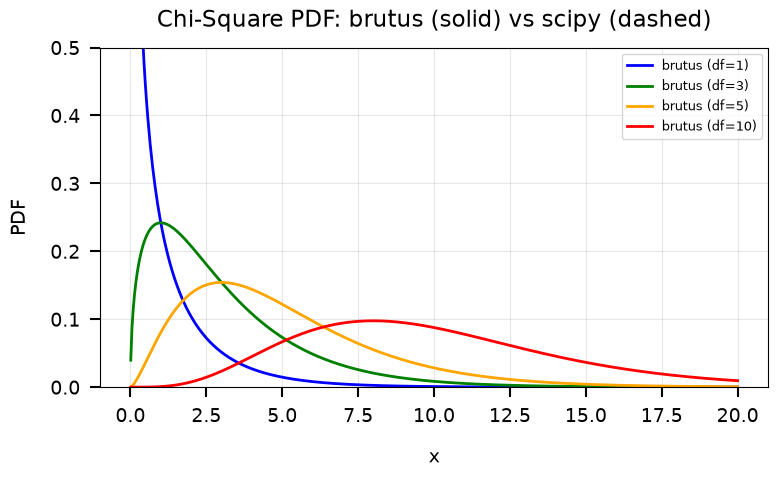
Max |log-PDF difference| for df=5: 1.78e-15
brutus and scipy chi-square log-PDFs agree to machine precision.

Show code cell source

Hide code cell source

from brutus.utils import truncnorm_pdf, truncnorm_logpdf
from scipy.stats import truncnorm as scipy_truncnorm

print_section("3d. Truncated Normal Distribution")

# Parameters: standard normal truncated to [-2, 3]
a, b = -2.0, 3.0
loc, scale = 0.0, 1.0

x = np.linspace(-4, 5, 500)

# brutus
pdf_brutus = truncnorm_pdf(x, a, b, loc=loc, scale=scale)
logpdf_brutus = truncnorm_logpdf(x, a, b, loc=loc, scale=scale)

# scipy (note: scipy uses standardized a, b limits)
a_std = (scale * a + loc - loc) / scale  # = a
b_std = (scale * b + loc - loc) / scale  # = b
pdf_scipy = scipy_truncnorm.pdf(x, a_std, b_std, loc=loc, scale=scale)
logpdf_scipy = scipy_truncnorm.logpdf(x, a_std, b_std, loc=loc, scale=scale)

fig, axes = plt.subplots(1, 2, figsize=(14, 5))

# Left: PDF comparison
ax = axes[0]
ax.plot(x, pdf_brutus, "b-", lw=2, label="brutus truncnorm_pdf")
ax.plot(x, pdf_scipy, "r--", lw=1.5, alpha=0.7, label="scipy truncnorm.pdf")
ax.axvline(scale * a + loc, color="gray", ls=":", lw=1.5, label=f"bounds [{scale*a+loc}, {scale*b+loc}]")
ax.axvline(scale * b + loc, color="gray", ls=":", lw=1.5)
ax.set_xlabel("x")
ax.set_ylabel("PDF")
ax.set_title("Truncated Normal PDF")
ax.legend(fontsize=9)
ax.grid(True, alpha=0.3)

# Right: log-PDF comparison
ax = axes[1]
ax.plot(x, logpdf_brutus, "b-", lw=2, label="brutus truncnorm_logpdf")
ax.plot(x, logpdf_scipy, "r--", lw=1.5, alpha=0.7, label="scipy truncnorm.logpdf")
ax.axvline(scale * a + loc, color="gray", ls=":", lw=1.5)
ax.axvline(scale * b + loc, color="gray", ls=":", lw=1.5)
ax.set_xlabel("x")
ax.set_ylabel("Log-PDF")
ax.set_title("Truncated Normal Log-PDF")
ax.set_ylim(-20, 2)
ax.legend(fontsize=9)
ax.grid(True, alpha=0.3)

save_figure(fig, 9, "truncnorm_comparison")
plt.show()

# Verify in the interior of the support
interior = (x > scale * a + loc + 0.01) & (x < scale * b + loc - 0.01)
max_pdf_diff = np.max(np.abs(pdf_brutus[interior] - pdf_scipy[interior]))
max_logpdf_diff = np.max(np.abs(logpdf_brutus[interior] - logpdf_scipy[interior]))

print(f"Max |PDF difference| in interior:     {max_pdf_diff:.2e}")
print(f"Max |log-PDF difference| in interior: {max_logpdf_diff:.2e}")
assert max_pdf_diff < 1e-10, f"Truncated normal PDF mismatch: {max_pdf_diff}"
assert max_logpdf_diff < 1e-10, f"Truncated normal log-PDF mismatch: {max_logpdf_diff}"
print("brutus and scipy truncated normal implementations agree.")

3d. Truncated Normal Distribution
=================================

  Saved: /mnt/c/Users/joshs/Dropbox/GitHub/brutus/tutorials/plots/tutorial_09/truncnorm_comparison.png

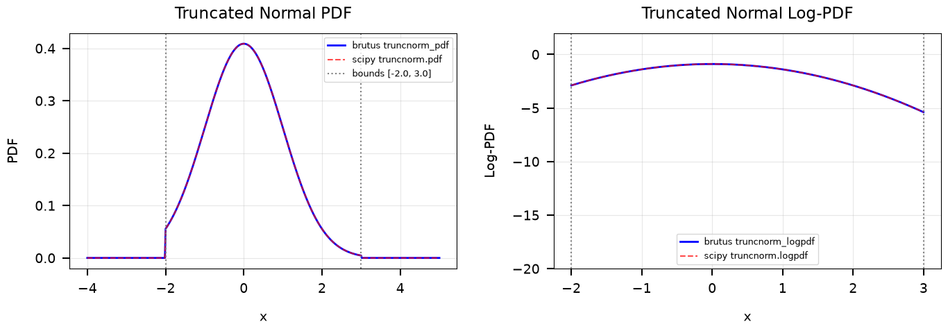
Max |PDF difference| in interior:     1.11e-16
Max |log-PDF difference| in interior: 0.00e+00
brutus and scipy truncated normal implementations agree.

4. Sampling Utilities

These functions are used for posterior analysis after fitting:

Function	Description
quantile	Compute (weighted) quantiles from samples
sample_multivariate_normal	Draw from multiple multivariate normals simultaneously
draw_sar	Draw from joint (scale, A_V, R_V) posterior

from brutus.utils import quantile

print_section("4a. Weighted Quantiles")

np.random.seed(77)

# Unweighted case
samples = np.sort(np.random.normal(5.0, 1.5, size=10000))
q_values = np.array([0.16, 0.50, 0.84])
q_unw = quantile(samples, q_values)

print("Unweighted samples (N=10000, mean=5, std=1.5):")
print(f"  16th percentile : {q_unw[0]:.3f}  (expected ~{5.0 - 1.5:.1f})")
print(f"  50th percentile : {q_unw[1]:.3f}  (expected ~5.0)")
print(f"  84th percentile : {q_unw[2]:.3f}  (expected ~{5.0 + 1.5:.1f})")

# Weighted case: heavily weight the upper tail
weights = np.where(samples > 6.0, 10.0, 1.0)
q_wt = quantile(samples, q_values, weights=weights)

print("\nWeighted samples (10x weight for samples > 6):")
print(f"  16th percentile : {q_wt[0]:.3f}")
print(f"  50th percentile : {q_wt[1]:.3f}")
print(f"  84th percentile : {q_wt[2]:.3f}")
print(f"\nWeighted median shifted from {q_unw[1]:.3f} to {q_wt[1]:.3f} (toward high values).")

assert_array_properties(q_unw, name="quantiles_unw", ndim=1, shape=(3,), finite=True)
assert_array_properties(q_wt, name="quantiles_wt", ndim=1, shape=(3,), finite=True)
assert q_wt[1] > q_unw[1], "Weighted median should be larger"
print("Quantile computations verified.")

4a. Weighted Quantiles
======================
Unweighted samples (N=10000, mean=5, std=1.5):
  16th percentile : 3.492  (expected ~3.5)
  50th percentile : 4.982  (expected ~5.0)
  84th percentile : 6.506  (expected ~6.5)

Weighted samples (10x weight for samples > 6):
  16th percentile : 5.077
  50th percentile : 6.482
  84th percentile : 7.480

Weighted median shifted from 4.982 to 6.482 (toward high values).
Quantile computations verified.

Show code cell source

Hide code cell source

from brutus.utils import sample_multivariate_normal

print_section("4b. Multivariate Normal Sampling")

np.random.seed(42)

# Define a 2D distribution with correlation
mean = np.array([3.0, -1.0])
cov = np.array([[1.0, 0.6],
                [0.6, 0.5]])

print(f"Mean: {mean}")
print(f"Covariance:\n{cov}")
print(f"isPSD(cov) = {isPSD(cov)}")

# Draw 2000 samples from a single distribution
Nsamples = 2000
samples_2d = sample_multivariate_normal(mean, cov, size=Nsamples)
print(f"\nSamples shape: {samples_2d.shape}  (dim, size)")

# Verify sample statistics
sample_mean = samples_2d.mean(axis=1)
sample_cov = np.cov(samples_2d)
print(f"\nSample mean: {sample_mean}  (expected: {mean})")
print(f"Sample cov:\n{sample_cov}")
print(f"(expected:\n{cov})")

assert_array_properties(samples_2d, name="mvn_samples", ndim=2, shape=(2, Nsamples), finite=True)

# Plot
fig, ax = plt.subplots(1, 1, figsize=(7, 6))
ax.scatter(samples_2d[0], samples_2d[1], s=3, alpha=0.3, color="steelblue")
ax.plot(mean[0], mean[1], "r+", markersize=15, mew=3, label="True mean")
ax.plot(sample_mean[0], sample_mean[1], "gx", markersize=12, mew=2, label="Sample mean")

# Draw 1-sigma ellipse
theta = np.linspace(0, 2 * np.pi, 200)
eigvals, eigvecs = np.linalg.eigh(cov)
circle = np.column_stack([np.cos(theta), np.sin(theta)])
ellipse = circle @ np.diag(np.sqrt(eigvals)) @ eigvecs.T + mean
ax.plot(ellipse[:, 0], ellipse[:, 1], "r-", lw=2, label=r"1$\sigma$ ellipse")

ax.set_xlabel("x")
ax.set_ylabel("y")
ax.set_title(f"Multivariate Normal Samples (N={Nsamples})")
ax.legend()
ax.set_aspect("equal")
ax.grid(True, alpha=0.3)

save_figure(fig, 9, "mvn_samples")
plt.show()

print("Sample distribution matches the specified mean and covariance.")

4b. Multivariate Normal Sampling
================================
Mean: [ 3. -1.]
Covariance:
[[1.  0.6]
 [0.6 0.5]]
isPSD(cov) = True

Samples shape: (2, 2000)  (dim, size)

Sample mean: [ 2.98417272 -1.00011614]  (expected: [ 3. -1.])
Sample cov:
[[0.9792843  0.57710111]
 [0.57710111 0.48133874]]
(expected:
[[1.  0.6]
 [0.6 0.5]])

  Saved: /mnt/c/Users/joshs/Dropbox/GitHub/brutus/tutorials/plots/tutorial_09/mvn_samples.png

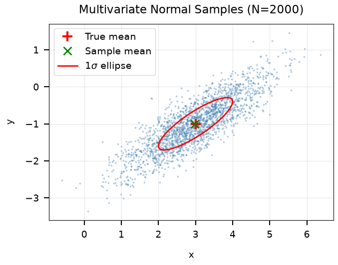
Sample distribution matches the specified mean and covariance.

4c. Scale Factor, Distance, and Extinction

The draw_sar function draws correlated samples of (scale, A_V, R_V) from the joint posterior at each model grid point. Understanding the scale factor is key to interpreting these draws:

• Scale represents the squared ratio of reference distance to true distance: scale = (d_ref / d)^2 = 1 / d_kpc^2 (since d_ref = 1 kpc in brutus).

• To convert a scale draw to a distance: d_kpc = 1 / sqrt(scale).

• Larger scale values correspond to closer objects; smaller scale values correspond to more distant objects.

Note that brutus now samples in log-distance space rather than scale-space in the main fitting pipeline. Log-distance sampling provides better importance sampling behavior, especially for distant or faint sources where the posterior in scale-space becomes highly skewed. The draw_sar utility remains available for cases where you need correlated (scale, A_V, R_V) draws from the per-model covariance matrices stored in BruteForce output.

What to look for in the plots below: The correlated (scale, A_V, R_V) draws illustrate how distance and extinction trade off – objects that are inferred to be closer (higher scale) tend to require less foreground extinction (lower A_V), and vice versa. The R_V draws show the additional uncertainty in the shape of the extinction curve.

Show code cell source

Hide code cell source

from brutus.utils import draw_sar

print_section("4c. Drawing from (Scale, A_V, R_V) Posterior")

np.random.seed(55)

# Simulate posterior parameters for 3 model grid points
Nsamps = 3
scales = np.array([1.0, 0.8, 1.2])     # scale factors
avs = np.array([0.5, 1.0, 2.0])        # A_V values
rvs = np.array([3.32, 3.3, 2.8])        # R_V values

# Covariance matrices (3x3 each)
covs_sar = np.zeros((Nsamps, 3, 3))
for i in range(Nsamps):
    L = np.diag([0.05, 0.1, 0.2])  # diagonal Cholesky factor
    L[1, 0] = 0.02  # small s-Av correlation
    L[2, 0] = 0.01  # small s-Rv correlation
    L[2, 1] = 0.05  # Av-Rv correlation
    covs_sar[i] = L @ L.T

print("Input parameters:")
for i in range(Nsamps):
    print(f"  Model {i}: scale={scales[i]:.2f}, A_V={avs[i]:.2f}, R_V={rvs[i]:.2f}")

# Generate draws
ndraws = 500
sdraws, adraws, rdraws = draw_sar(
    scales, avs, rvs, covs_sar, ndraws=ndraws,
    avlim=(0.0, 6.0), rvlim=(1.0, 8.0)
)

print(f"\nDraw shapes: scale={sdraws.shape}, A_V={adraws.shape}, R_V={rdraws.shape}")

assert_array_properties(sdraws, name="scale_draws", ndim=2, shape=(Nsamps, ndraws), finite=True)
assert_array_properties(adraws, name="av_draws", ndim=2, shape=(Nsamps, ndraws), finite=True,
                        min_val=0.0, max_val=6.0)
assert_array_properties(rdraws, name="rv_draws", ndim=2, shape=(Nsamps, ndraws), finite=True,
                        min_val=1.0, max_val=8.0)
print("All draws within specified bounds (A_V: [0, 6], R_V: [1, 8]).")

# Plot the draws
fig, axes = plt.subplots(1, 3, figsize=(16, 5))

param_names = ["Scale", r"$A_V$", r"$R_V$"]
draw_arrays = [sdraws, adraws, rdraws]
true_vals = [scales, avs, rvs]
colors = ["steelblue", "darkorange", "seagreen"]

for col, (ax, pname, draws, trues) in enumerate(
    zip(axes, param_names, draw_arrays, true_vals)
):
    for i in range(Nsamps):
        ax.hist(draws[i], bins=40, alpha=0.5, density=True,
                color=colors[i], label=f"Model {i} (true={trues[i]:.1f})")
        ax.axvline(trues[i], color=colors[i], ls="--", lw=2)
    ax.set_xlabel(pname)
    ax.set_ylabel("Density")
    ax.set_title(f"{pname} Posterior Draws")
    ax.legend(fontsize=8)
    ax.grid(True, alpha=0.3)

plt.suptitle(f"draw_sar: {ndraws} draws per model, rejection-sampled within bounds",
             fontsize=13)
save_figure(fig, 9, "draw_sar")
plt.show()

print("Draws are centered on input values and respect physical bounds.")

4c. Drawing from (Scale, A_V, R_V) Posterior
============================================
Input parameters:
  Model 0: scale=1.00, A_V=0.50, R_V=3.32
  Model 1: scale=0.80, A_V=1.00, R_V=3.30
  Model 2: scale=1.20, A_V=2.00, R_V=2.80

Draw shapes: scale=(3, 500), A_V=(3, 500), R_V=(3, 500)
All draws within specified bounds (A_V: [0, 6], R_V: [1, 8]).

  Saved: /mnt/c/Users/joshs/Dropbox/GitHub/brutus/tutorials/plots/tutorial_09/draw_sar.png

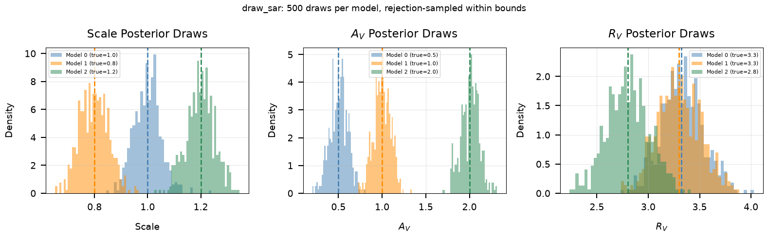
Draws are centered on input values and respect physical bounds.

Summary

This tutorial demonstrated the utility functions available in brutus.utils:

Photometry Conversions (Section 1)

• magnitude / inv_magnitude provide exact round-trip conversion between flux and AB magnitudes.

• luptitude / inv_luptitude provide asinh magnitudes that remain well-behaved at faint fluxes where standard magnitudes diverge.

• add_mag combines fluxes expressed as magnitudes.

Photometric Likelihoods (Section 2)

• phot_loglike is the core likelihood function used in BruteForce fitting. The optional dim_prior flag adds a chi-square dimensionality penalty.

• chisquare_outlier_loglike and uniform_outlier_loglike provide baseline log-likelihoods for identifying outlier objects that no stellar model can fit.

Mathematical Utilities (Section 3)

• inverse3 provides fast, numba-accelerated 3x3 matrix inversion optimized for covariance matrices.

• isPSD checks whether a matrix is positive semi-definite, which is required for valid covariance matrices.

• chisquare_logpdf and truncnorm_pdf / truncnorm_logpdf replicate scipy distributions with lightweight implementations.

Sampling Utilities (Section 4)

• quantile computes weighted quantiles from posterior samples, essential for credible intervals.

• sample_multivariate_normal draws from many multivariate normal distributions simultaneously using Cholesky decomposition.

• draw_sar generates rejection-sampled posterior draws for (scale, A_V, R_V) within physical bounds.

Next Steps

These utilities are used throughout the brutus fitting pipeline. See:

• Tutorial 5 for how phot_loglike drives the BruteForce fitter

• Tutorial 6 for how draw_sar and quantile appear in cluster analysis

• Tutorial 8 for how photometric offsets interact with magnitude conversions