Tutorial 7: 3D Dust Mapping

Tutorial 7: 3D Dust Mapping#

This tutorial demonstrates line-of-sight dust modeling with brutus, fitting multi-cloud models to stellar distance-extinction posteriors using nested sampling.

Topics Covered#

Loading stellar posteriors for distance and extinction
Line-of-sight dust modeling with multi-cloud models
LOS dust fitting with nested sampling (dynesty)

Prerequisites#

This tutorial optionally uses:

Stellar posterior samples from Tutorial 5

The tutorial will generate synthetic data if these files are not available.

Requirement: the line-of-sight fitting sections use the dynesty nested sampler, which is not a brutus dependency — install it with pip install dynesty before running this tutorial.

# Imports and setup
import numpy as np
import matplotlib.pyplot as plt
from pathlib import Path
import warnings
warnings.filterwarnings('ignore')
import h5py

# Import tutorial utilities
from tutorial_utils import (
    set_plot_style,
    find_brutus_data_file,
    save_figure as save_fig_util,
)

# Set plot style
set_plot_style()
plt.rcParams['figure.figsize'] = (10, 6)

# Create plots directory if needed
plots_dir = Path('plots/tutorial_07')
plots_dir.mkdir(parents=True, exist_ok=True)

def save_figure(fig, name):
    """Helper to save figures."""
    filepath = plots_dir / f"{name}.png"
    fig.savefig(filepath, dpi=150, bbox_inches='tight')
    print(f"  Saved: {filepath}")

Line-of-Sight Dust Modeling#

Real dust distributions often have discrete cloud structures along the line of sight. The brutus.analysis.los_dust module provides tools to fit multi-cloud models to stellar extinction measurements, decomposing the cumulative extinction into a foreground component plus discrete cloud jumps at specific distances.

Input Data#

The LOS fitter works with posterior samples from BruteForce fits. Each star contributes distance and extinction samples that collectively trace the distance-reddening relation along the sightline.

Let’s load stellar posteriors and examine the distance-extinction structure.

Note: The LOS dust fitting in this tutorial uses the dynesty nested sampling package. Install it with pip install dynesty if you don’t have it already.

# Try to load real stellar posterior samples or generate synthetic ones
print("Preparing stellar posterior samples for LOS dust modeling...\n")

try:
    # Try to find results from Tutorial 5 (Orion field, no-dust-prior fit)
    datafile = Path('Orion_l209.1_b-19.9_mist_nodust.h5')

    if not datafile.exists():
        datafile = find_brutus_data_file("Orion_l209.1_b-19.9_mist_nodust.h5")

    with h5py.File(datafile, 'r') as f:
        # Load distance and extinction samples
        dist_samples = f['samps_dist'][:] if 'samps_dist' in f else None
        av_samples = f['samps_red'][:] if 'samps_red' in f else None
        chi2 = f['obj_chi2min'][:] if 'obj_chi2min' in f else None
        nbands = f['obj_Nbands'][:] if 'obj_Nbands' in f else None

        if dist_samples is not None and av_samples is not None:
            print(f"Loaded {len(dist_samples)} stellar posterior samples from file")

            # Apply a loose chi2 cut to remove poor fits
            if chi2 is not None and nbands is not None:
                from scipy.stats import chi2 as chi2_dist
                # Goodness-of-fit p-value, not chi2/Nbands.
                dof = np.maximum(nbands - 3, 1)
                pvals = chi2_dist.sf(chi2, dof)
                good = pvals > 1e-6  # drop only the worst fits
                dist_samples = dist_samples[good]
                av_samples = av_samples[good]
                print(f"  After p-value > 1e-6 cut: {len(dist_samples)} stars kept")

            # Convert distances to distance modulus for LOS fitting
            dm_samples = 5 * np.log10(dist_samples * 1000) - 5  # kpc to distance modulus

            source = "Real Data"
        else:
            raise ValueError("No distance/extinction samples in file")

            

except (FileNotFoundError, ValueError, KeyError) as e:

    # Generate synthetic samples
    print("Generating synthetic stellar samples...")
    print(f"  (Real data not available: {e})\n")
    
    n_stars = 50
    n_samples = 100

    # Create synthetic distance modulus samples
    # Simulate stars at various distances with measurement uncertainties
    true_dm = np.random.uniform(7, 10, n_stars)  # True distance moduli
    dm_error = np.random.uniform(0.1, 0.3, n_stars)  # Uncertainties

    dm_samples = np.zeros((n_stars, n_samples))
    for i in range(n_stars):
        dm_samples[i] = np.random.normal(true_dm[i], dm_error[i], n_samples)

    # Create synthetic extinction samples (correlated with distance)
    # Simulate a dust cloud at distance modulus ~8.5
    cloud_dm = 8.5
    cloud_width = 0.3

    av_samples = np.zeros((n_stars, n_samples))
    for i in range(n_stars):
        # Background extinction
        av_bg = 0.3

        # Add cloud extinction for stars behind it
        for j in range(n_samples):
            if dm_samples[i, j] > cloud_dm:
                av_cloud = 1.5 * (1 - np.exp(-(dm_samples[i, j] - cloud_dm) / cloud_width))
                av_samples[i, j] = av_bg + av_cloud + np.random.normal(0, 0.1)
            else:
                av_samples[i, j] = av_bg * (dm_samples[i, j] / cloud_dm) + np.random.normal(0, 0.1)

    av_samples = np.maximum(0, av_samples)  # No negative extinction
    source = "Synthetic"

print(f"Using {source} stellar samples:")
print(f"  Stars: {len(dm_samples)}")
print(f"  Samples per star: {dm_samples.shape[1]}")
print(f"  Distance modulus range: [{dm_samples.min():.1f}, {dm_samples.max():.1f}]")
print(f"  A_V range: [{av_samples.min():.2f}, {av_samples.max():.2f}] mag")

Preparing stellar posterior samples for LOS dust modeling...

Loaded 207 stellar posterior samples from file

  After p-value > 1e-6 cut: 138 stars kept
Using Real Data stellar samples:
  Stars: 138
  Samples per star: 500
  Distance modulus range: [7.1, 21.2]
  A_V range: [0.00, 5.95] mag

Show code cell source

Hide code cell source

# Distance-extinction relation from stellar posteriors
from brutus.plotting import bin_pdfs_distred

# --- Bin posteriors into 2D distance-reddening PDFs ---
# bin_pdfs_distred expects (n_objects, n_samples) arrays for distance (in kpc)
# and reddening. We pass (dists, reds, dreds) as a 3-tuple.
dist_kpc = 10**((dm_samples + 5) / 5) / 1000  # DM -> kpc
rv_dummy = 3.32 * np.ones_like(av_samples)  # placeholder R(V)

# Determine plot span from data
dm_lo, dm_hi = float(np.nanmin(dm_samples)) - 0.5, float(np.nanmax(dm_samples)) + 0.5
av_lo, av_hi = 0.0, max(2.0, float(np.nanmax(av_samples)) + 0.3)
dist_lo = 10**((dm_lo + 5) / 5) / 1000
dist_hi = 10**((dm_hi + 5) / 5) / 1000

binned, xedges, yedges = bin_pdfs_distred(
    (dist_kpc, av_samples, rv_dummy),
    dist_type='distance_modulus',
    avlim=(av_lo, av_hi),
    span=((av_lo, av_hi), (dist_lo, dist_hi)),
    bins=(300, 150),
    smooth=0.02,
)
# binned shape: (n_stars, n_xbins, n_ybins) where x=DM, y=A_V

# Compute bin centers
xc = 0.5 * (xedges[:-1] + xedges[1:])  # distance modulus
yc = 0.5 * (yedges[:-1] + yedges[1:])  # A_V

# --- Build stacked 2D density (sum over all stars) ---
stacked = binned.sum(axis=0)

# --- Plot: single panel only (no marginals) ---
fig, ax_main = plt.subplots(figsize=(10, 6))

# Main panel: stacked 2D density + scatter
ax_main.pcolormesh(xedges, yedges, stacked.T, cmap='Greys', alpha=0.7)

# Overlay per-star medians
dm_median = np.median(dm_samples, axis=1)
dm_std = np.std(dm_samples, axis=1)
av_median = np.median(av_samples, axis=1)
av_std = np.std(av_samples, axis=1)
ax_main.errorbar(dm_median, av_median, xerr=dm_std, yerr=av_std,
                 fmt='none', ecolor='gray', alpha=0.3, zorder=1)
ax_main.scatter(dm_median, av_median, c='steelblue', s=20, zorder=5,
                edgecolor='k', linewidth=0.3)
ax_main.set_xlabel('Distance Modulus')
ax_main.set_ylabel('$A_V$ (mag)')
ax_main.set_ylim(bottom=0)
ax_main.grid(True, alpha=0.3)

fig.suptitle(f'Distance-Extinction Relation ({source})', fontsize=14, fontweight='bold')
plt.tight_layout()
save_figure(fig, 'stellar_samples')
plt.show()

print(f"Stars: {len(dm_median)}, DM range: [{dm_median.min():.1f}, {dm_median.max():.1f}]")
print(f"A_V range: [{av_median.min():.2f}, {av_median.max():.2f}] mag")

  Saved: plots/tutorial_07/stellar_samples.png

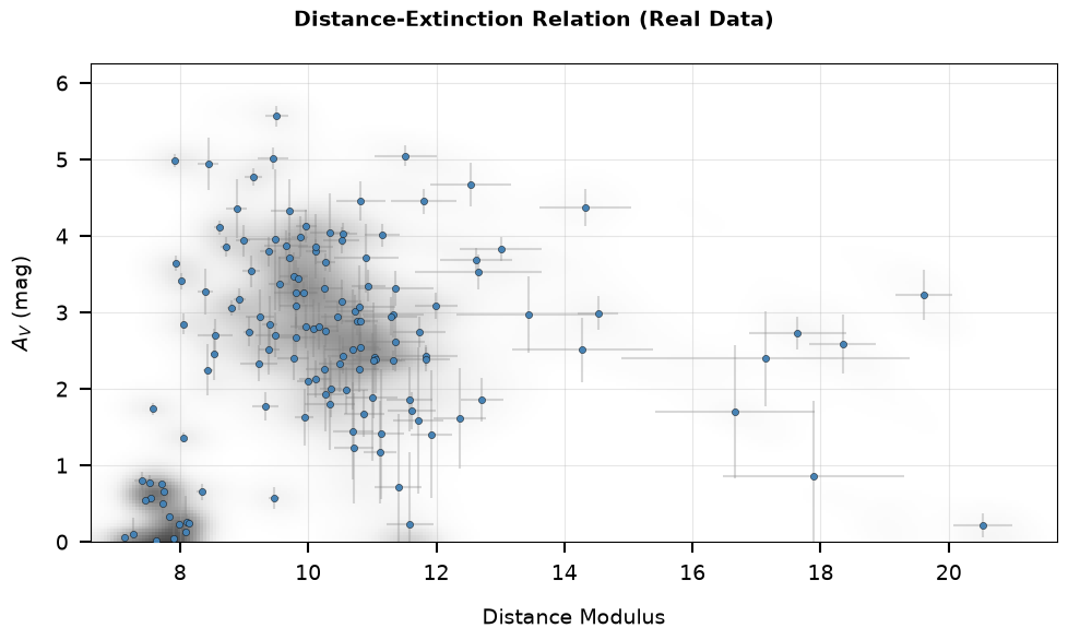
../_images/c3b39b2b4be5b04453a3eaa5e95b48ecb9e1ac6224141b78149987cd88bccc0d.png

Stars: 138, DM range: [7.1, 20.5]
A_V range: [0.02, 5.57] mag

Fitting a LOS Dust Model with Dynesty#

The LOS fitter uses two key functions designed for nested sampling:

los_clouds_priortransform(u, rlims, dlims): Transforms unit cube draws into physical parameters. For an $n$-cloud model the parameter vector has $2n + 4$ elements: $[p_b, s_{\text{fore}}, s_{\text{back}}, A_{V,\text{fore}}, d_1, A_{V,1}, \ldots, d_n, A_{V,n}]$
los_clouds_loglike_samples(theta, dsamps, rsamps, ...): Log-likelihood of the cloud model given stellar distance/reddening posterior samples.

For a 1-cloud model (ndim=6), the parameters are:

Parameter	Meaning
$p_b$	Outlier fraction
$s_{\text{fore}}$	Foreground smoothing scale
$s_{\text{back}}$	Background smoothing scale
$A_{V,\text{fore}}$	Foreground extinction (before cloud)
$d_1$	Cloud distance (distance modulus)
$A_{V,1}$	Total extinction (after cloud)

Let’s run a real nested sampling fit on the stellar posteriors.

# Run LOS dust fit with dynesty
from brutus.analysis import los_clouds_priortransform, los_clouds_loglike_samples
import dynesty
from dynesty.utils import resample_equal

# Set up 1-cloud model (ndim = 6)
ndim = 6

# Determine appropriate bounds from the data
dm_range = (float(dm_samples.min()) - 0.5, float(dm_samples.max()) + 0.5)
av_range = (0.0, max(3.0, float(av_samples.max()) + 0.5))

print(f"LOS fit setup:")
print(f"  Model: 1-cloud ({ndim} parameters)")
print(f"  Stars: {dm_samples.shape[0]}")
print(f"  Samples per star: {dm_samples.shape[1]}")
print(f"  Distance modulus bounds: [{dm_range[0]:.1f}, {dm_range[1]:.1f}]")
print(f"  A_V bounds: [{av_range[0]:.1f}, {av_range[1]:.1f}]")

def prior_transform(u):
    return los_clouds_priortransform(u, rlims=av_range, dlims=dm_range)

def loglike(theta):
    return los_clouds_loglike_samples(
        theta, dm_samples, av_samples,
        kernel='gauss', rlims=av_range, Ndraws=25, monotonic=True
    )

# Run nested sampling (rslice sampler is more efficient for this problem)
import time
print("\nRunning nested sampling...")
t0 = time.time()
sampler = dynesty.NestedSampler(loglike, prior_transform, ndim,
                                nlive=200, sample='rslice')
sampler.run_nested(print_progress=True, maxcall=250000)
results = sampler.results
t_run = time.time() - t0

print(f"  Completed in {t_run:.1f}s")
print(f"  Log-evidence: {results.logz[-1]:.1f} +/- {results.logzerr[-1]:.1f}")
print(f"  Iterations: {results.niter}")

# Extract weighted posterior
weights = np.exp(results.logwt - results.logz[-1])
weights /= weights.sum()
posterior = resample_equal(results.samples, weights)

param_names = ['P_b', 's_fore', 's_back', 'A_V_fore', 'd_cloud (DM)', 'A_V_total']
print(f"\nPosterior summary (median [16th, 84th]):")
for i, name in enumerate(param_names):
    med = np.median(posterior[:, i])
    lo, hi = np.percentile(posterior[:, i], [16, 84])
    print(f"  {name:20s}: {med:.3f}  [{lo:.3f}, {hi:.3f}]")

# Convert cloud distance to kpc
dm_cloud = np.median(posterior[:, 4])
dist_kpc = 10**((dm_cloud + 5) / 5) / 1000
delta_av = np.median(posterior[:, 5] - posterior[:, 3])
print(f"\nCloud properties:")
print(f"  Distance: {dist_kpc:.2f} kpc (DM = {dm_cloud:.1f})")
print(f"  Foreground A_V: {np.median(posterior[:, 3]):.3f} mag")
print(f"  Extinction jump at cloud: {delta_av:.3f} mag")

LOS fit setup:
  Model: 1-cloud (6 parameters)
  Stars: 138
  Samples per star: 500
  Distance modulus bounds: [6.6, 21.7]
  A_V bounds: [0.0, 6.5]

Running nested sampling...

0it [00:00, ?it/s]

56it [00:00, 559.73it/s, bound: 0 | nc: 2 | ncall: 322 | eff(%): 17.391 | loglstar:   -inf <   -inf <    inf | logz:   -inf +/-    nan | dlogz:    inf >  0.209]

112it [00:00, 556.13it/s, bound: 0 | nc: 2 | ncall: 423 | eff(%): 26.478 | loglstar:   -inf < -598.787 <    inf | logz: -605.482 +/-    nan | dlogz: 355.807 >  0.209]

168it [00:00, 453.85it/s, bound: 0 | nc: 1 | ncall: 580 | eff(%): 28.966 | loglstar:   -inf < -511.578 <    inf | logz: -517.823 +/-    nan | dlogz: 284.026 >  0.209]

216it [00:00, 399.70it/s, bound: 0 | nc: 2 | ncall: 770 | eff(%): 28.052 | loglstar:   -inf < -467.003 <    inf | logz: -473.540 +/-    nan | dlogz: 239.950 >  0.209]

258it [00:00, 374.63it/s, bound: 0 | nc: 1 | ncall: 929 | eff(%): 27.772 | loglstar:   -inf < -442.350 <    inf | logz: -448.205 +/-    nan | dlogz: 213.642 >  0.209]

297it [00:00, 344.96it/s, bound: 0 | nc: 8 | ncall: 1082 | eff(%): 27.449 | loglstar:   -inf < -416.461 <    inf | logz: -422.500 +/-    nan | dlogz: 187.584 >  0.209]

333it [00:00, 315.02it/s, bound: 0 | nc: 7 | ncall: 1264 | eff(%): 26.345 | loglstar:   -inf < -393.767 <    inf | logz: -400.483 +/-    nan | dlogz: 165.660 >  0.209]

366it [00:01, 255.53it/s, bound: 0 | nc: 5 | ncall: 1527 | eff(%): 23.969 | loglstar:   -inf < -378.125 <    inf | logz: -383.892 +/-    nan | dlogz: 148.466 >  0.209]

394it [00:01, 225.86it/s, bound: 0 | nc: 2 | ncall: 1764 | eff(%): 22.336 | loglstar:   -inf < -362.677 <    inf | logz: -368.985 +/-    nan | dlogz: 133.611 >  0.209]

418it [00:01, 169.47it/s, bound: 0 | nc: 13 | ncall: 2104 | eff(%): 19.867 | loglstar:   -inf < -355.170 <    inf | logz: -361.194 +/-    nan | dlogz: 125.540 >  0.209]

438it [00:01, 142.51it/s, bound: 0 | nc: 34 | ncall: 2403 | eff(%): 18.227 | loglstar:   -inf < -349.675 <    inf | logz: -355.720 +/-    nan | dlogz: 119.945 >  0.209]

455it [00:01, 135.24it/s, bound: 0 | nc: 10 | ncall: 2639 | eff(%): 17.241 | loglstar:   -inf < -346.334 <    inf | logz: -352.442 +/-    nan | dlogz: 116.563 >  0.209]

470it [00:02, 114.08it/s, bound: 0 | nc: 2 | ncall: 2956 | eff(%): 15.900 | loglstar:   -inf < -341.951 <    inf | logz: -348.293 +/-    nan | dlogz: 112.382 >  0.209] 

485it [00:02, 119.23it/s, bound: 0 | nc: 6 | ncall: 3095 | eff(%): 15.670 | loglstar:   -inf < -338.823 <    inf | logz: -344.822 +/-    nan | dlogz: 108.761 >  0.209]

498it [00:02, 104.44it/s, bound: 0 | nc: 23 | ncall: 3354 | eff(%): 14.848 | loglstar:   -inf < -335.593 <    inf | logz: -341.616 +/-    nan | dlogz: 105.485 >  0.209]

510it [00:02, 92.30it/s, bound: 0 | nc: 3 | ncall: 3615 | eff(%): 14.108 | loglstar:   -inf < -332.961 <    inf | logz: -339.450 +/-    nan | dlogz: 103.288 >  0.209]  

520it [00:02, 85.90it/s, bound: 0 | nc: 8 | ncall: 3822 | eff(%): 13.605 | loglstar:   -inf < -331.548 <    inf | logz: -337.787 +/-    nan | dlogz: 101.551 >  0.209]

529it [00:02, 75.96it/s, bound: 0 | nc: 35 | ncall: 4089 | eff(%): 12.937 | loglstar:   -inf < -330.066 <    inf | logz: -336.350 +/-    nan | dlogz: 100.060 >  0.209]

540it [00:02, 81.73it/s, bound: 0 | nc: 16 | ncall: 4241 | eff(%): 12.733 | loglstar:   -inf < -326.489 <    inf | logz: -333.403 +/-    nan | dlogz: 97.197 >  0.209] 

549it [00:03, 72.93it/s, bound: 0 | nc: 17 | ncall: 4492 | eff(%): 12.222 | loglstar:   -inf < -324.377 <    inf | logz: -331.147 +/-    nan | dlogz: 101.497 >  0.209]

557it [00:03, 66.77it/s, bound: 0 | nc: 69 | ncall: 4716 | eff(%): 11.811 | loglstar:   -inf < -321.579 <    inf | logz: -328.397 +/-    nan | dlogz: 98.717 >  0.209] 

564it [00:03, 66.16it/s, bound: 0 | nc: 32 | ncall: 4888 | eff(%): 11.538 | loglstar:   -inf < -319.789 <    inf | logz: -326.637 +/-    nan | dlogz: 96.912 >  0.209]

571it [00:03, 63.00it/s, bound: 0 | nc: 2 | ncall: 5100 | eff(%): 11.196 | loglstar:   -inf < -318.761 <    inf | logz: -325.187 +/-    nan | dlogz: 95.321 >  0.209] 

578it [00:03, 64.06it/s, bound: 0 | nc: 9 | ncall: 5238 | eff(%): 11.035 | loglstar:   -inf < -317.452 <    inf | logz: -324.221 +/-    nan | dlogz: 94.346 >  0.209]

585it [00:03, 61.64it/s, bound: 0 | nc: 2 | ncall: 5398 | eff(%): 10.837 | loglstar:   -inf < -316.257 <    inf | logz: -322.925 +/-    nan | dlogz: 93.023 >  0.209]

592it [00:03, 59.18it/s, bound: 0 | nc: 1 | ncall: 5592 | eff(%): 10.587 | loglstar:   -inf < -315.205 <    inf | logz: -321.754 +/-    nan | dlogz: 91.788 >  0.209]

598it [00:04, 52.86it/s, bound: 0 | nc: 9 | ncall: 5798 | eff(%): 10.314 | loglstar:   -inf < -313.971 <    inf | logz: -320.635 +/-    nan | dlogz: 90.652 >  0.209]

605it [00:04, 56.12it/s, bound: 0 | nc: 25 | ncall: 5956 | eff(%): 10.158 | loglstar:   -inf < -312.732 <    inf | logz: -319.441 +/-    nan | dlogz: 89.432 >  0.209]

611it [00:04, 48.35it/s, bound: 1 | nc: 48 | ncall: 6207 | eff(%):  9.844 | loglstar:   -inf < -311.546 <    inf | logz: -318.321 +/-    nan | dlogz: 88.292 >  0.209]

617it [00:04, 38.63it/s, bound: 1 | nc: 52 | ncall: 6485 | eff(%):  9.514 | loglstar:   -inf < -311.119 <    inf | logz: -317.485 +/-    nan | dlogz: 87.350 >  0.209]

622it [00:04, 31.02it/s, bound: 1 | nc: 43 | ncall: 6734 | eff(%):  9.237 | loglstar:   -inf < -310.268 <    inf | logz: -316.743 +/-    nan | dlogz: 86.587 >  0.209]

626it [00:05, 27.17it/s, bound: 1 | nc: 48 | ncall: 6929 | eff(%):  9.034 | loglstar:   -inf < -309.148 <    inf | logz: -316.018 +/-    nan | dlogz: 85.892 >  0.209]

630it [00:05, 25.22it/s, bound: 1 | nc: 48 | ncall: 7124 | eff(%):  8.843 | loglstar:   -inf < -308.605 <    inf | logz: -315.293 +/-    nan | dlogz: 85.134 >  0.209]

633it [00:05, 23.68it/s, bound: 1 | nc: 51 | ncall: 7281 | eff(%):  8.694 | loglstar:   -inf < -308.428 <    inf | logz: -314.898 +/-    nan | dlogz: 84.684 >  0.209]

636it [00:05, 22.77it/s, bound: 1 | nc: 49 | ncall: 7429 | eff(%):  8.561 | loglstar:   -inf < -307.982 <    inf | logz: -314.499 +/-    nan | dlogz: 84.275 >  0.209]

639it [00:05, 22.67it/s, bound: 1 | nc: 48 | ncall: 7571 | eff(%):  8.440 | loglstar:   -inf < -307.741 <    inf | logz: -314.153 +/-    nan | dlogz: 83.897 >  0.209]

642it [00:05, 22.74it/s, bound: 1 | nc: 52 | ncall: 7726 | eff(%):  8.310 | loglstar:   -inf < -307.505 <    inf | logz: -313.846 +/-    nan | dlogz: 83.564 >  0.209]

645it [00:05, 21.38it/s, bound: 1 | nc: 56 | ncall: 7891 | eff(%):  8.174 | loglstar:   -inf < -306.765 <    inf | logz: -313.509 +/-    nan | dlogz: 83.244 >  0.209]

648it [00:06, 20.92it/s, bound: 2 | nc: 46 | ncall: 8043 | eff(%):  8.057 | loglstar:   -inf < -306.313 <    inf | logz: -313.105 +/-    nan | dlogz: 82.833 >  0.209]

651it [00:06, 22.19it/s, bound: 2 | nc: 57 | ncall: 8192 | eff(%):  7.947 | loglstar:   -inf < -306.157 <    inf | logz: -312.704 +/-    nan | dlogz: 82.397 >  0.209]

654it [00:06, 19.73it/s, bound: 2 | nc: 53 | ncall: 8386 | eff(%):  7.799 | loglstar:   -inf < -305.642 <    inf | logz: -312.308 +/-    nan | dlogz: 81.995 >  0.209]

657it [00:06, 20.80it/s, bound: 2 | nc: 47 | ncall: 8529 | eff(%):  7.703 | loglstar:   -inf < -305.253 <    inf | logz: -311.899 +/-    nan | dlogz: 81.573 >  0.209]

660it [00:06, 20.86it/s, bound: 2 | nc: 49 | ncall: 8683 | eff(%):  7.601 | loglstar:   -inf < -304.776 <    inf | logz: -311.486 +/-    nan | dlogz: 81.147 >  0.209]

663it [00:06, 22.05it/s, bound: 2 | nc: 45 | ncall: 8816 | eff(%):  7.520 | loglstar:   -inf < -304.609 <    inf | logz: -311.140 +/-    nan | dlogz: 80.762 >  0.209]

666it [00:06, 22.66it/s, bound: 2 | nc: 48 | ncall: 8969 | eff(%):  7.426 | loglstar:   -inf < -304.023 <    inf | logz: -310.824 +/-    nan | dlogz: 92.753 >  0.209]

669it [00:07, 23.40it/s, bound: 2 | nc: 52 | ncall: 9115 | eff(%):  7.340 | loglstar:   -inf < -303.613 <    inf | logz: -310.405 +/-    nan | dlogz: 92.339 >  0.209]

672it [00:07, 24.53it/s, bound: 2 | nc: 53 | ncall: 9257 | eff(%):  7.259 | loglstar:   -inf < -303.146 <    inf | logz: -310.008 +/-    nan | dlogz: 91.925 >  0.209]

675it [00:07, 23.99it/s, bound: 2 | nc: 54 | ncall: 9411 | eff(%):  7.172 | loglstar:   -inf < -302.725 <    inf | logz: -309.591 +/-    nan | dlogz: 91.500 >  0.209]

678it [00:07, 23.43it/s, bound: 2 | nc: 47 | ncall: 9550 | eff(%):  7.099 | loglstar:   -inf < -302.138 <    inf | logz: -309.107 +/-    nan | dlogz: 91.025 >  0.209]

681it [00:07, 22.63it/s, bound: 2 | nc: 53 | ncall: 9704 | eff(%):  7.018 | loglstar:   -inf < -301.676 <    inf | logz: -308.602 +/-    nan | dlogz: 90.493 >  0.209]

684it [00:07, 22.47it/s, bound: 3 | nc: 50 | ncall: 9851 | eff(%):  6.943 | loglstar:   -inf < -301.270 <    inf | logz: -308.159 +/-    nan | dlogz: 90.024 >  0.209]

687it [00:07, 22.16it/s, bound: 3 | nc: 54 | ncall: 10002 | eff(%):  6.869 | loglstar:   -inf < -300.905 <    inf | logz: -307.731 +/-    nan | dlogz: 89.571 >  0.209]

690it [00:08, 21.57it/s, bound: 3 | nc: 51 | ncall: 10147 | eff(%):  6.800 | loglstar:   -inf < -300.782 <    inf | logz: -307.390 +/-    nan | dlogz: 89.188 >  0.209]

693it [00:08, 22.34it/s, bound: 3 | nc: 54 | ncall: 10288 | eff(%):  6.736 | loglstar:   -inf < -299.929 <    inf | logz: -306.987 +/-    nan | dlogz: 88.825 >  0.209]

696it [00:08, 23.04it/s, bound: 3 | nc: 72 | ncall: 10441 | eff(%):  6.666 | loglstar:   -inf < -299.672 <    inf | logz: -306.567 +/-    nan | dlogz: 89.135 >  0.209]

699it [00:08, 20.82it/s, bound: 3 | nc: 72 | ncall: 10619 | eff(%):  6.583 | loglstar:   -inf < -299.453 <    inf | logz: -306.201 +/-    nan | dlogz: 88.735 >  0.209]

702it [00:08, 20.87it/s, bound: 3 | nc: 54 | ncall: 10772 | eff(%):  6.517 | loglstar:   -inf < -299.164 <    inf | logz: -305.883 +/-    nan | dlogz: 88.390 >  0.209]

705it [00:08, 20.04it/s, bound: 3 | nc: 54 | ncall: 10962 | eff(%):  6.431 | loglstar:   -inf < -298.468 <    inf | logz: -305.478 +/-    nan | dlogz: 88.006 >  0.209]

708it [00:08, 20.29it/s, bound: 3 | nc: 49 | ncall: 11128 | eff(%):  6.362 | loglstar:   -inf < -298.417 <    inf | logz: -305.114 +/-    nan | dlogz: 87.596 >  0.209]

711it [00:09, 19.20it/s, bound: 3 | nc: 43 | ncall: 11299 | eff(%):  6.293 | loglstar:   -inf < -298.183 <    inf | logz: -304.801 +/-    nan | dlogz: 87.257 >  0.209]

714it [00:09, 20.95it/s, bound: 3 | nc: 39 | ncall: 11436 | eff(%):  6.243 | loglstar:   -inf < -297.519 <    inf | logz: -304.429 +/-    nan | dlogz: 86.902 >  0.209]

717it [00:09, 18.38it/s, bound: 4 | nc: 44 | ncall: 11621 | eff(%):  6.170 | loglstar:   -inf < -297.018 <    inf | logz: -304.028 +/-    nan | dlogz: 86.493 >  0.209]

720it [00:09, 20.20it/s, bound: 4 | nc: 41 | ncall: 11759 | eff(%):  6.123 | loglstar:   -inf < -296.537 <    inf | logz: -303.592 +/-    nan | dlogz: 86.046 >  0.209]

723it [00:09, 21.26it/s, bound: 4 | nc: 49 | ncall: 11903 | eff(%):  6.074 | loglstar:   -inf < -296.298 <    inf | logz: -303.204 +/-    nan | dlogz: 85.622 >  0.209]

726it [00:09, 21.54it/s, bound: 4 | nc: 46 | ncall: 12056 | eff(%):  6.022 | loglstar:   -inf < -295.780 <    inf | logz: -302.783 +/-    nan | dlogz: 85.200 >  0.209]

729it [00:09, 22.03it/s, bound: 4 | nc: 45 | ncall: 12204 | eff(%):  5.973 | loglstar:   -inf < -294.975 <    inf | logz: -302.286 +/-    nan | dlogz: 84.739 >  0.209]

732it [00:10, 21.43it/s, bound: 4 | nc: 53 | ncall: 12360 | eff(%):  5.922 | loglstar:   -inf < -294.030 <    inf | logz: -301.613 +/-    nan | dlogz: 84.100 >  0.209]

735it [00:10, 22.01it/s, bound: 4 | nc: 47 | ncall: 12503 | eff(%):  5.879 | loglstar:   -inf < -293.547 <    inf | logz: -301.018 +/-    nan | dlogz: 83.455 >  0.209]

738it [00:10, 23.12it/s, bound: 4 | nc: 38 | ncall: 12637 | eff(%):  5.840 | loglstar:   -inf < -293.325 <    inf | logz: -300.511 +/-    nan | dlogz: 82.890 >  0.209]

741it [00:10, 22.16it/s, bound: 4 | nc: 78 | ncall: 12828 | eff(%):  5.776 | loglstar:   -inf < -293.200 <    inf | logz: -300.138 +/-    nan | dlogz: 82.460 >  0.209]

744it [00:10, 18.98it/s, bound: 4 | nc: 60 | ncall: 13031 | eff(%):  5.709 | loglstar:   -inf < -292.789 <    inf | logz: -299.801 +/-    nan | dlogz: 82.111 >  0.209]

747it [00:10, 19.61it/s, bound: 4 | nc: 51 | ncall: 13188 | eff(%):  5.664 | loglstar:   -inf < -292.580 <    inf | logz: -299.482 +/-    nan | dlogz: 81.764 >  0.209]

750it [00:10, 18.44it/s, bound: 4 | nc: 99 | ncall: 13381 | eff(%):  5.605 | loglstar:   -inf < -291.819 <    inf | logz: -299.149 +/-    nan | dlogz: 81.444 >  0.209]

752it [00:11, 18.65it/s, bound: 5 | nc: 42 | ncall: 13480 | eff(%):  5.579 | loglstar:   -inf < -291.460 <    inf | logz: -298.805 +/-    nan | dlogz: 81.130 >  0.209]

755it [00:11, 20.27it/s, bound: 5 | nc: 47 | ncall: 13624 | eff(%):  5.542 | loglstar:   -inf < -291.213 <    inf | logz: -298.381 +/-    nan | dlogz: 80.655 >  0.209]

758it [00:11, 21.15it/s, bound: 5 | nc: 48 | ncall: 13779 | eff(%):  5.501 | loglstar:   -inf < -291.025 <    inf | logz: -298.028 +/-    nan | dlogz: 80.264 >  0.209]

761it [00:11, 20.54it/s, bound: 5 | nc: 59 | ncall: 13941 | eff(%):  5.459 | loglstar:   -inf < -290.869 <    inf | logz: -297.721 +/-    nan | dlogz: 79.925 >  0.209]

764it [00:11, 20.85it/s, bound: 5 | nc: 53 | ncall: 14093 | eff(%):  5.421 | loglstar:   -inf < -290.499 <    inf | logz: -297.437 +/-    nan | dlogz: 79.627 >  0.209]

767it [00:11, 21.79it/s, bound: 5 | nc: 57 | ncall: 14247 | eff(%):  5.384 | loglstar:   -inf < -290.191 <    inf | logz: -297.148 +/-    nan | dlogz: 79.326 >  0.209]

770it [00:11, 20.52it/s, bound: 5 | nc: 59 | ncall: 14432 | eff(%):  5.335 | loglstar:   -inf < -289.812 <    inf | logz: -296.838 +/-    nan | dlogz: 79.004 >  0.209]

773it [00:12, 20.61it/s, bound: 5 | nc: 48 | ncall: 14586 | eff(%):  5.300 | loglstar:   -inf < -289.424 <    inf | logz: -296.508 +/-    nan | dlogz: 78.664 >  0.209]

776it [00:12, 20.85it/s, bound: 5 | nc: 54 | ncall: 14753 | eff(%):  5.260 | loglstar:   -inf < -289.019 <    inf | logz: -296.190 +/-    nan | dlogz: 78.334 >  0.209]

779it [00:12, 21.04it/s, bound: 5 | nc: 55 | ncall: 14926 | eff(%):  5.219 | loglstar:   -inf < -288.716 <    inf | logz: -295.853 +/-    nan | dlogz: 77.985 >  0.209]

782it [00:12, 21.20it/s, bound: 5 | nc: 42 | ncall: 15079 | eff(%):  5.186 | loglstar:   -inf < -288.381 <    inf | logz: -295.525 +/-    nan | dlogz: 77.639 >  0.209]

785it [00:12, 22.01it/s, bound: 5 | nc: 48 | ncall: 15228 | eff(%):  5.155 | loglstar:   -inf < -288.210 <    inf | logz: -295.208 +/-    nan | dlogz: 77.295 >  0.209]

788it [00:12, 20.91it/s, bound: 6 | nc: 50 | ncall: 15374 | eff(%):  5.126 | loglstar:   -inf < -287.943 <    inf | logz: -294.930 +/-    nan | dlogz: 76.998 >  0.209]

791it [00:12, 22.09it/s, bound: 6 | nc: 62 | ncall: 15552 | eff(%):  5.086 | loglstar:   -inf < -287.795 <    inf | logz: -294.674 +/-    nan | dlogz: 76.716 >  0.209]

794it [00:13, 20.43it/s, bound: 6 | nc: 61 | ncall: 15743 | eff(%):  5.044 | loglstar:   -inf < -287.694 <    inf | logz: -294.446 +/-    nan | dlogz: 76.462 >  0.209]

797it [00:13, 20.80it/s, bound: 6 | nc: 61 | ncall: 15909 | eff(%):  5.010 | loglstar:   -inf < -287.300 <    inf | logz: -294.224 +/-    nan | dlogz: 76.230 >  0.209]

800it [00:13, 21.12it/s, bound: 6 | nc: 48 | ncall: 16068 | eff(%):  4.979 | loglstar:   -inf < -287.026 <    inf | logz: -293.977 +/-    nan | dlogz: 75.977 >  0.209]

803it [00:13, 22.43it/s, bound: 6 | nc: 45 | ncall: 16209 | eff(%):  4.954 | loglstar:   -inf < -286.674 <    inf | logz: -293.706 +/-    nan | dlogz: 75.699 >  0.209]

806it [00:13, 22.85it/s, bound: 6 | nc: 54 | ncall: 16364 | eff(%):  4.925 | loglstar:   -inf < -286.288 <    inf | logz: -293.421 +/-    nan | dlogz: 75.401 >  0.209]

809it [00:13, 20.48it/s, bound: 6 | nc: 56 | ncall: 16560 | eff(%):  4.885 | loglstar:   -inf < -286.161 <    inf | logz: -293.155 +/-    nan | dlogz: 75.109 >  0.209]

812it [00:13, 20.93it/s, bound: 6 | nc: 45 | ncall: 16712 | eff(%):  4.859 | loglstar:   -inf < -285.869 <    inf | logz: -292.907 +/-    nan | dlogz: 74.845 >  0.209]

815it [00:14, 19.98it/s, bound: 6 | nc: 78 | ncall: 16909 | eff(%):  4.820 | loglstar:   -inf < -285.535 <    inf | logz: -292.653 +/-    nan | dlogz: 74.580 >  0.209]

818it [00:14, 18.97it/s, bound: 7 | nc: 59 | ncall: 17089 | eff(%):  4.787 | loglstar:   -inf < -285.372 <    inf | logz: -292.398 +/-    nan | dlogz: 74.305 >  0.209]

820it [00:14, 17.74it/s, bound: 7 | nc: 65 | ncall: 17208 | eff(%):  4.765 | loglstar:   -inf < -285.299 <    inf | logz: -292.242 +/-    nan | dlogz: 74.133 >  0.209]

823it [00:14, 19.34it/s, bound: 7 | nc: 43 | ncall: 17356 | eff(%):  4.742 | loglstar:   -inf < -285.063 <    inf | logz: -292.024 +/-    nan | dlogz: 73.897 >  0.209]

825it [00:14, 17.57it/s, bound: 7 | nc: 61 | ncall: 17504 | eff(%):  4.713 | loglstar:   -inf < -284.967 <    inf | logz: -291.879 +/-    nan | dlogz: 73.740 >  0.209]

828it [00:14, 19.35it/s, bound: 7 | nc: 45 | ncall: 17641 | eff(%):  4.694 | loglstar:   -inf < -284.892 <    inf | logz: -291.681 +/-    nan | dlogz: 73.518 >  0.209]

831it [00:14, 19.85it/s, bound: 7 | nc: 54 | ncall: 17797 | eff(%):  4.669 | loglstar:   -inf < -284.508 <    inf | logz: -291.468 +/-    nan | dlogz: 73.300 >  0.209]

834it [00:15, 20.99it/s, bound: 7 | nc: 47 | ncall: 17936 | eff(%):  4.650 | loglstar:   -inf < -284.074 <    inf | logz: -291.222 +/-    nan | dlogz: 73.050 >  0.209]

837it [00:15, 21.72it/s, bound: 7 | nc: 48 | ncall: 18074 | eff(%):  4.631 | loglstar:   -inf < -284.067 <    inf | logz: -290.994 +/-    nan | dlogz: 72.794 >  0.209]

840it [00:15, 20.97it/s, bound: 7 | nc: 60 | ncall: 18235 | eff(%):  4.607 | loglstar:   -inf < -283.820 <    inf | logz: -290.780 +/-    nan | dlogz: 72.565 >  0.209]

843it [00:15, 21.24it/s, bound: 7 | nc: 56 | ncall: 18384 | eff(%):  4.586 | loglstar:   -inf < -283.682 <    inf | logz: -290.583 +/-    nan | dlogz: 72.347 >  0.209]

846it [00:15, 22.01it/s, bound: 7 | nc: 60 | ncall: 18523 | eff(%):  4.567 | loglstar:   -inf < -282.943 <    inf | logz: -290.357 +/-    nan | dlogz: 72.135 >  0.209]

849it [00:15, 22.35it/s, bound: 7 | nc: 50 | ncall: 18672 | eff(%):  4.547 | loglstar:   -inf < -282.440 <    inf | logz: -290.041 +/-    nan | dlogz: 71.826 >  0.209]

852it [00:15, 21.50it/s, bound: 7 | nc: 47 | ncall: 18829 | eff(%):  4.525 | loglstar:   -inf < -282.203 <    inf | logz: -289.699 +/-    nan | dlogz: 71.464 >  0.209]

855it [00:15, 20.27it/s, bound: 8 | nc: 55 | ncall: 18992 | eff(%):  4.502 | loglstar:   -inf < -281.942 <    inf | logz: -289.364 +/-    nan | dlogz: 71.110 >  0.209]

858it [00:16, 20.47it/s, bound: 8 | nc: 57 | ncall: 19149 | eff(%):  4.481 | loglstar:   -inf < -281.706 <    inf | logz: -289.064 +/-    nan | dlogz: 71.902 >  0.209]

861it [00:16, 20.09it/s, bound: 8 | nc: 57 | ncall: 19324 | eff(%):  4.456 | loglstar:   -inf < -281.525 <    inf | logz: -288.788 +/-    nan | dlogz: 71.604 >  0.209]

864it [00:16, 20.07it/s, bound: 8 | nc: 43 | ncall: 19474 | eff(%):  4.437 | loglstar:   -inf < -281.311 <    inf | logz: -288.535 +/-    nan | dlogz: 71.331 >  0.209]

867it [00:16, 20.39it/s, bound: 8 | nc: 55 | ncall: 19636 | eff(%):  4.415 | loglstar:   -inf < -281.109 <    inf | logz: -288.295 +/-    nan | dlogz: 71.071 >  0.209]

870it [00:16, 19.98it/s, bound: 8 | nc: 58 | ncall: 19797 | eff(%):  4.395 | loglstar:   -inf < -280.771 <    inf | logz: -288.062 +/-    nan | dlogz: 70.825 >  0.209]

873it [00:16, 21.54it/s, bound: 8 | nc: 40 | ncall: 19925 | eff(%):  4.381 | loglstar:   -inf < -280.155 <    inf | logz: -287.770 +/-    nan | dlogz: 70.542 >  0.209]

876it [00:17, 21.05it/s, bound: 8 | nc: 60 | ncall: 20087 | eff(%):  4.361 | loglstar:   -inf < -280.033 <    inf | logz: -287.462 +/-    nan | dlogz: 70.211 >  0.209]

879it [00:17, 21.47it/s, bound: 8 | nc: 43 | ncall: 20226 | eff(%):  4.346 | loglstar:   -inf < -279.643 <    inf | logz: -287.172 +/-    nan | dlogz: 69.909 >  0.209]

882it [00:17, 22.09it/s, bound: 8 | nc: 44 | ncall: 20371 | eff(%):  4.330 | loglstar:   -inf < -279.517 <    inf | logz: -286.902 +/-    nan | dlogz: 69.611 >  0.209]

885it [00:17, 22.19it/s, bound: 8 | nc: 47 | ncall: 20512 | eff(%):  4.315 | loglstar:   -inf < -279.355 <    inf | logz: -286.664 +/-    nan | dlogz: 69.350 >  0.209]

888it [00:17, 22.18it/s, bound: 8 | nc: 40 | ncall: 20652 | eff(%):  4.300 | loglstar:   -inf < -279.101 <    inf | logz: -286.429 +/-    nan | dlogz: 69.100 >  0.209]

891it [00:17, 21.90it/s, bound: 9 | nc: 52 | ncall: 20797 | eff(%):  4.284 | loglstar:   -inf < -278.263 <    inf | logz: -286.097 +/-    nan | dlogz: 68.797 >  0.209]

894it [00:17, 21.99it/s, bound: 9 | nc: 42 | ncall: 20949 | eff(%):  4.268 | loglstar:   -inf < -278.105 <    inf | logz: -285.739 +/-    nan | dlogz: 68.412 >  0.209]

897it [00:18, 18.73it/s, bound: 9 | nc: 51 | ncall: 21159 | eff(%):  4.239 | loglstar:   -inf < -277.984 <    inf | logz: -285.450 +/-    nan | dlogz: 68.089 >  0.209]

900it [00:18, 19.74it/s, bound: 9 | nc: 52 | ncall: 21305 | eff(%):  4.224 | loglstar:   -inf < -277.830 <    inf | logz: -285.209 +/-    nan | dlogz: 67.820 >  0.209]

903it [00:18, 18.92it/s, bound: 9 | nc: 56 | ncall: 21489 | eff(%):  4.202 | loglstar:   -inf < -277.629 <    inf | logz: -284.987 +/-    nan | dlogz: 67.580 >  0.209]

906it [00:18, 19.84it/s, bound: 9 | nc: 61 | ncall: 21642 | eff(%):  4.186 | loglstar:   -inf < -277.457 <    inf | logz: -284.770 +/-    nan | dlogz: 67.345 >  0.209]

909it [00:18, 20.26it/s, bound: 9 | nc: 52 | ncall: 21796 | eff(%):  4.170 | loglstar:   -inf < -276.869 <    inf | logz: -284.509 +/-    nan | dlogz: 67.098 >  0.209]

912it [00:18, 20.16it/s, bound: 9 | nc: 54 | ncall: 21946 | eff(%):  4.156 | loglstar:   -inf < -276.717 <    inf | logz: -284.241 +/-    nan | dlogz: 66.802 >  0.209]

915it [00:18, 21.24it/s, bound: 9 | nc: 46 | ncall: 22099 | eff(%):  4.140 | loglstar:   -inf < -276.519 <    inf | logz: -283.988 +/-    nan | dlogz: 66.528 >  0.209]

918it [00:19, 20.74it/s, bound: 9 | nc: 60 | ncall: 22246 | eff(%):  4.127 | loglstar:   -inf < -275.988 <    inf | logz: -283.696 +/-    nan | dlogz: 66.244 >  0.209]

921it [00:19, 20.23it/s, bound: 9 | nc: 48 | ncall: 22409 | eff(%):  4.110 | loglstar:   -inf < -275.682 <    inf | logz: -283.409 +/-    nan | dlogz: 65.937 >  0.209]

924it [00:19, 18.59it/s, bound: 10 | nc: 52 | ncall: 22574 | eff(%):  4.093 | loglstar:   -inf < -275.382 <    inf | logz: -283.119 +/-    nan | dlogz: 65.629 >  0.209]

927it [00:19, 19.63it/s, bound: 10 | nc: 57 | ncall: 22720 | eff(%):  4.080 | loglstar:   -inf < -274.847 <    inf | logz: -282.802 +/-    nan | dlogz: 65.318 >  0.209]

930it [00:19, 19.77it/s, bound: 10 | nc: 52 | ncall: 22886 | eff(%):  4.064 | loglstar:   -inf < -274.340 <    inf | logz: -282.402 +/-    nan | dlogz: 64.922 >  0.209]

933it [00:19, 19.75it/s, bound: 10 | nc: 56 | ncall: 23042 | eff(%):  4.049 | loglstar:   -inf < -274.137 <    inf | logz: -282.045 +/-    nan | dlogz: 64.529 >  0.209]

935it [00:19, 19.65it/s, bound: 10 | nc: 49 | ncall: 23140 | eff(%):  4.041 | loglstar:   -inf < -274.079 <    inf | logz: -281.836 +/-    nan | dlogz: 64.296 >  0.209]

938it [00:20, 18.56it/s, bound: 10 | nc: 76 | ncall: 23323 | eff(%):  4.022 | loglstar:   -inf < -274.023 <    inf | logz: -281.583 +/-    nan | dlogz: 64.007 >  0.209]

940it [00:20, 18.38it/s, bound: 10 | nc: 56 | ncall: 23433 | eff(%):  4.011 | loglstar:   -inf < -273.841 <    inf | logz: -281.423 +/-    nan | dlogz: 63.838 >  0.209]

942it [00:20, 18.04it/s, bound: 10 | nc: 55 | ncall: 23550 | eff(%):  4.000 | loglstar:   -inf < -273.539 <    inf | logz: -281.257 +/-    nan | dlogz: 63.667 >  0.209]

944it [00:20, 17.88it/s, bound: 10 | nc: 59 | ncall: 23662 | eff(%):  3.990 | loglstar:   -inf < -273.245 <    inf | logz: -281.063 +/-    nan | dlogz: 63.476 >  0.209]

947it [00:20, 19.48it/s, bound: 10 | nc: 50 | ncall: 23807 | eff(%):  3.978 | loglstar:   -inf < -273.151 <    inf | logz: -280.798 +/-    nan | dlogz: 63.181 >  0.209]

950it [00:20, 20.20it/s, bound: 10 | nc: 55 | ncall: 23944 | eff(%):  3.968 | loglstar:   -inf < -272.873 <    inf | logz: -280.552 +/-    nan | dlogz: 62.920 >  0.209]

953it [00:20, 21.49it/s, bound: 10 | nc: 51 | ncall: 24080 | eff(%):  3.958 | loglstar:   -inf < -272.523 <    inf | logz: -280.313 +/-    nan | dlogz: 62.667 >  0.209]

956it [00:20, 21.26it/s, bound: 10 | nc: 55 | ncall: 24238 | eff(%):  3.944 | loglstar:   -inf < -272.280 <    inf | logz: -280.047 +/-    nan | dlogz: 62.391 >  0.209]

959it [00:21, 21.03it/s, bound: 11 | nc: 45 | ncall: 24377 | eff(%):  3.934 | loglstar:   -inf < -272.152 <    inf | logz: -279.800 +/-    nan | dlogz: 62.118 >  0.209]

962it [00:21, 22.58it/s, bound: 11 | nc: 39 | ncall: 24506 | eff(%):  3.926 | loglstar:   -inf < -271.834 <    inf | logz: -279.566 +/-    nan | dlogz: 61.869 >  0.209]

965it [00:21, 20.92it/s, bound: 11 | nc: 57 | ncall: 24665 | eff(%):  3.912 | loglstar:   -inf < -271.684 <    inf | logz: -279.334 +/-    nan | dlogz: 61.619 >  0.209]

968it [00:21, 21.24it/s, bound: 11 | nc: 55 | ncall: 24812 | eff(%):  3.901 | loglstar:   -inf < -271.171 <    inf | logz: -279.083 +/-    nan | dlogz: 61.369 >  0.209]

971it [00:21, 21.64it/s, bound: 11 | nc: 53 | ncall: 24962 | eff(%):  3.890 | loglstar:   -inf < -270.931 <    inf | logz: -278.798 +/-    nan | dlogz: 61.070 >  0.209]

974it [00:21, 21.84it/s, bound: 11 | nc: 44 | ncall: 25109 | eff(%):  3.879 | loglstar:   -inf < -270.795 <    inf | logz: -278.544 +/-    nan | dlogz: 60.789 >  0.209]

977it [00:21, 20.19it/s, bound: 11 | nc: 49 | ncall: 25277 | eff(%):  3.865 | loglstar:   -inf < -270.559 <    inf | logz: -278.311 +/-    nan | dlogz: 60.541 >  0.209]

980it [00:22, 19.62it/s, bound: 11 | nc: 54 | ncall: 25426 | eff(%):  3.854 | loglstar:   -inf < -270.425 <    inf | logz: -278.093 +/-    nan | dlogz: 60.299 >  0.209]

983it [00:22, 20.89it/s, bound: 11 | nc: 41 | ncall: 25555 | eff(%):  3.847 | loglstar:   -inf < -270.080 <    inf | logz: -277.885 +/-    nan | dlogz: 60.078 >  0.209]

986it [00:22, 21.03it/s, bound: 11 | nc: 48 | ncall: 25704 | eff(%):  3.836 | loglstar:   -inf < -269.896 <    inf | logz: -277.656 +/-    nan | dlogz: 59.835 >  0.209]

989it [00:22, 21.08it/s, bound: 11 | nc: 63 | ncall: 25856 | eff(%):  3.825 | loglstar:   -inf < -269.615 <    inf | logz: -277.434 +/-    nan | dlogz: 59.601 >  0.209]

992it [00:22, 20.52it/s, bound: 11 | nc: 57 | ncall: 26018 | eff(%):  3.813 | loglstar:   -inf < -269.269 <    inf | logz: -277.170 +/-    nan | dlogz: 59.331 >  0.209]

995it [00:22, 20.22it/s, bound: 11 | nc: 56 | ncall: 26171 | eff(%):  3.802 | loglstar:   -inf < -269.070 <    inf | logz: -276.929 +/-    nan | dlogz: 59.067 >  0.209]

998it [00:23, 19.93it/s, bound: 12 | nc: 48 | ncall: 26326 | eff(%):  3.791 | loglstar:   -inf < -268.749 <    inf | logz: -276.687 +/-    nan | dlogz: 58.817 >  0.209]

1001it [00:23, 17.75it/s, bound: 12 | nc: 61 | ncall: 26539 | eff(%):  3.772 | loglstar:   -inf < -268.621 <    inf | logz: -276.456 +/-    nan | dlogz: 58.560 >  0.209]

1004it [00:23, 18.92it/s, bound: 12 | nc: 42 | ncall: 26676 | eff(%):  3.764 | loglstar:   -inf < -268.298 <    inf | logz: -276.222 +/-    nan | dlogz: 58.316 >  0.209]

1006it [00:23, 19.05it/s, bound: 12 | nc: 58 | ncall: 26785 | eff(%):  3.756 | loglstar:   -inf < -268.218 <    inf | logz: -276.069 +/-    nan | dlogz: 58.149 >  0.209]

1009it [00:23, 20.37it/s, bound: 12 | nc: 36 | ncall: 26917 | eff(%):  3.749 | loglstar:   -inf < -268.140 <    inf | logz: -275.867 +/-    nan | dlogz: 57.922 >  0.209]

1012it [00:23, 20.64it/s, bound: 12 | nc: 45 | ncall: 27066 | eff(%):  3.739 | loglstar:   -inf < -267.756 <    inf | logz: -275.653 +/-    nan | dlogz: 57.706 >  0.209]

1015it [00:23, 20.11it/s, bound: 12 | nc: 60 | ncall: 27221 | eff(%):  3.729 | loglstar:   -inf < -267.354 <    inf | logz: -275.404 +/-    nan | dlogz: 57.453 >  0.209]

1018it [00:24, 19.44it/s, bound: 12 | nc: 48 | ncall: 27391 | eff(%):  3.717 | loglstar:   -inf < -267.247 <    inf | logz: -275.167 +/-    nan | dlogz: 57.189 >  0.209]

1020it [00:24, 18.41it/s, bound: 12 | nc: 72 | ncall: 27517 | eff(%):  3.707 | loglstar:   -inf < -266.806 <    inf | logz: -275.003 +/-    nan | dlogz: 57.026 >  0.209]

1022it [00:24, 17.06it/s, bound: 12 | nc: 57 | ncall: 27641 | eff(%):  3.697 | loglstar:   -inf < -266.643 <    inf | logz: -274.809 +/-    nan | dlogz: 56.830 >  0.209]

1025it [00:24, 18.00it/s, bound: 12 | nc: 48 | ncall: 27801 | eff(%):  3.687 | loglstar:   -inf < -266.435 <    inf | logz: -274.548 +/-    nan | dlogz: 56.545 >  0.209]

1027it [00:24, 17.35it/s, bound: 12 | nc: 88 | ncall: 27936 | eff(%):  3.676 | loglstar:   -inf < -266.408 <    inf | logz: -274.387 +/-    nan | dlogz: 56.365 >  0.209]

1029it [00:24, 16.27it/s, bound: 13 | nc: 40 | ncall: 28054 | eff(%):  3.668 | loglstar:   -inf < -266.202 <    inf | logz: -274.235 +/-    nan | dlogz: 56.203 >  0.209]

1031it [00:24, 17.07it/s, bound: 13 | nc: 63 | ncall: 28159 | eff(%):  3.661 | loglstar:   -inf < -266.134 <    inf | logz: -274.087 +/-    nan | dlogz: 56.040 >  0.209]

1034it [00:24, 18.83it/s, bound: 13 | nc: 48 | ncall: 28304 | eff(%):  3.653 | loglstar:   -inf < -265.918 <    inf | logz: -273.864 +/-    nan | dlogz: 55.803 >  0.209]

1036it [00:25, 18.50it/s, bound: 13 | nc: 63 | ncall: 28406 | eff(%):  3.647 | loglstar:   -inf < -265.778 <    inf | logz: -273.725 +/-    nan | dlogz: 55.651 >  0.209]

1039it [00:25, 19.46it/s, bound: 13 | nc: 56 | ncall: 28559 | eff(%):  3.638 | loglstar:   -inf < -265.348 <    inf | logz: -273.489 +/-    nan | dlogz: 55.411 >  0.209]

1041it [00:25, 18.97it/s, bound: 13 | nc: 50 | ncall: 28664 | eff(%):  3.632 | loglstar:   -inf < -265.050 <    inf | logz: -273.305 +/-    nan | dlogz: 55.230 >  0.209]

1043it [00:25, 18.96it/s, bound: 13 | nc: 45 | ncall: 28763 | eff(%):  3.626 | loglstar:   -inf < -264.626 <    inf | logz: -273.106 +/-    nan | dlogz: 55.032 >  0.209]

1045it [00:25, 18.13it/s, bound: 13 | nc: 59 | ncall: 28870 | eff(%):  3.620 | loglstar:   -inf < -264.588 <    inf | logz: -272.897 +/-    nan | dlogz: 54.808 >  0.209]

1048it [00:25, 17.33it/s, bound: 13 | nc: 87 | ncall: 29064 | eff(%):  3.606 | loglstar:   -inf < -264.178 <    inf | logz: -272.588 +/-    nan | dlogz: 54.489 >  0.209]

1050it [00:25, 16.39it/s, bound: 13 | nc: 56 | ncall: 29195 | eff(%):  3.597 | loglstar:   -inf < -264.030 <    inf | logz: -272.385 +/-    nan | dlogz: 54.270 >  0.209]

1052it [00:26, 16.49it/s, bound: 13 | nc: 79 | ncall: 29318 | eff(%):  3.588 | loglstar:   -inf < -263.923 <    inf | logz: -272.201 +/-    nan | dlogz: 54.067 >  0.209]

1054it [00:26, 16.19it/s, bound: 13 | nc: 50 | ncall: 29437 | eff(%):  3.581 | loglstar:   -inf < -263.760 <    inf | logz: -272.019 +/-    nan | dlogz: 53.875 >  0.209]

1056it [00:26, 16.97it/s, bound: 13 | nc: 53 | ncall: 29541 | eff(%):  3.575 | loglstar:   -inf < -263.735 <    inf | logz: -271.858 +/-    nan | dlogz: 53.692 >  0.209]

1058it [00:26, 17.03it/s, bound: 13 | nc: 57 | ncall: 29639 | eff(%):  3.570 | loglstar:   -inf < -263.399 <    inf | logz: -271.703 +/-    nan | dlogz: 53.530 >  0.209]

1061it [00:26, 18.51it/s, bound: 13 | nc: 63 | ncall: 29798 | eff(%):  3.561 | loglstar:   -inf < -263.145 <    inf | logz: -271.429 +/-    nan | dlogz: 53.248 >  0.209]

1063it [00:26, 17.38it/s, bound: 14 | nc: 64 | ncall: 29908 | eff(%):  3.554 | loglstar:   -inf < -262.864 <    inf | logz: -271.243 +/-    nan | dlogz: 53.058 >  0.209]

1065it [00:26, 17.44it/s, bound: 14 | nc: 68 | ncall: 30027 | eff(%):  3.547 | loglstar:   -inf < -262.526 <    inf | logz: -271.047 +/-    nan | dlogz: 52.859 >  0.209]

1067it [00:26, 16.92it/s, bound: 14 | nc: 54 | ncall: 30145 | eff(%):  3.540 | loglstar:   -inf < -262.440 <    inf | logz: -270.847 +/-    nan | dlogz: 52.645 >  0.209]

1070it [00:27, 19.00it/s, bound: 14 | nc: 47 | ncall: 30296 | eff(%):  3.532 | loglstar:   -inf < -262.300 <    inf | logz: -270.579 +/-    nan | dlogz: 52.351 >  0.209]

1072it [00:27, 18.82it/s, bound: 14 | nc: 54 | ncall: 30401 | eff(%):  3.526 | loglstar:   -inf < -261.976 <    inf | logz: -270.415 +/-    nan | dlogz: 52.177 >  0.209]

1074it [00:27, 17.88it/s, bound: 14 | nc: 56 | ncall: 30511 | eff(%):  3.520 | loglstar:   -inf < -261.963 <    inf | logz: -270.240 +/-    nan | dlogz: 51.990 >  0.209]

1077it [00:27, 20.08it/s, bound: 14 | nc: 51 | ncall: 30671 | eff(%):  3.511 | loglstar:   -inf < -261.661 <    inf | logz: -269.995 +/-    nan | dlogz: 51.730 >  0.209]

1080it [00:27, 21.24it/s, bound: 14 | nc: 57 | ncall: 30813 | eff(%):  3.505 | loglstar:   -inf < -261.429 <    inf | logz: -269.737 +/-    nan | dlogz: 51.456 >  0.209]

1083it [00:27, 18.54it/s, bound: 14 | nc: 50 | ncall: 30999 | eff(%):  3.494 | loglstar:   -inf < -261.368 <    inf | logz: -269.517 +/-    nan | dlogz: 51.208 >  0.209]

1085it [00:27, 18.57it/s, bound: 14 | nc: 57 | ncall: 31103 | eff(%):  3.488 | loglstar:   -inf < -261.172 <    inf | logz: -269.383 +/-    nan | dlogz: 51.062 >  0.209]

1088it [00:27, 19.52it/s, bound: 14 | nc: 50 | ncall: 31257 | eff(%):  3.481 | loglstar:   -inf < -260.913 <    inf | logz: -269.166 +/-    nan | dlogz: 50.834 >  0.209]

1090it [00:28, 18.18it/s, bound: 14 | nc: 54 | ncall: 31385 | eff(%):  3.473 | loglstar:   -inf < -260.760 <    inf | logz: -269.025 +/-    nan | dlogz: 50.682 >  0.209]

1092it [00:28, 18.39it/s, bound: 14 | nc: 48 | ncall: 31492 | eff(%):  3.468 | loglstar:   -inf < -260.742 <    inf | logz: -268.888 +/-    nan | dlogz: 50.531 >  0.209]

1095it [00:28, 19.96it/s, bound: 14 | nc: 54 | ncall: 31637 | eff(%):  3.461 | loglstar:   -inf < -260.679 <    inf | logz: -268.707 +/-    nan | dlogz: 50.326 >  0.209]

1098it [00:28, 19.23it/s, bound: 15 | nc: 58 | ncall: 31787 | eff(%):  3.454 | loglstar:   -inf < -260.575 <    inf | logz: -268.541 +/-    nan | dlogz: 50.141 >  0.209]

1100it [00:28, 17.06it/s, bound: 15 | nc: 79 | ncall: 31932 | eff(%):  3.445 | loglstar:   -inf < -260.526 <    inf | logz: -268.440 +/-    nan | dlogz: 50.026 >  0.209]

1102it [00:28, 17.62it/s, bound: 15 | nc: 45 | ncall: 32026 | eff(%):  3.441 | loglstar:   -inf < -260.159 <    inf | logz: -268.329 +/-    nan | dlogz: 49.914 >  0.209]

1105it [00:28, 18.54it/s, bound: 15 | nc: 54 | ncall: 32181 | eff(%):  3.434 | loglstar:   -inf < -260.042 <    inf | logz: -268.150 +/-    nan | dlogz: 49.720 >  0.209]

1107it [00:28, 18.40it/s, bound: 15 | nc: 59 | ncall: 32290 | eff(%):  3.428 | loglstar:   -inf < -259.536 <    inf | logz: -267.996 +/-    nan | dlogz: 49.580 >  0.209]

1110it [00:29, 19.47it/s, bound: 15 | nc: 59 | ncall: 32448 | eff(%):  3.421 | loglstar:   -inf < -259.171 <    inf | logz: -267.717 +/-    nan | dlogz: 49.294 >  0.209]

1112it [00:29, 18.87it/s, bound: 15 | nc: 48 | ncall: 32551 | eff(%):  3.416 | loglstar:   -inf < -259.069 <    inf | logz: -267.548 +/-    nan | dlogz: 49.107 >  0.209]

1114it [00:29, 18.30it/s, bound: 15 | nc: 66 | ncall: 32667 | eff(%):  3.410 | loglstar:   -inf < -258.956 <    inf | logz: -267.392 +/-    nan | dlogz: 48.936 >  0.209]

1117it [00:29, 18.18it/s, bound: 15 | nc: 82 | ncall: 32840 | eff(%):  3.401 | loglstar:   -inf < -258.488 <    inf | logz: -267.146 +/-    nan | dlogz: 48.685 >  0.209]

1120it [00:29, 16.40it/s, bound: 15 | nc: 127 | ncall: 33057 | eff(%):  3.388 | loglstar:   -inf < -258.290 <    inf | logz: -266.884 +/-    nan | dlogz: 48.405 >  0.209]

1122it [00:29, 16.94it/s, bound: 15 | nc: 66 | ncall: 33174 | eff(%):  3.382 | loglstar:   -inf < -258.013 <    inf | logz: -266.690 +/-    nan | dlogz: 51.118 >  0.209] 

1124it [00:29, 16.09it/s, bound: 15 | nc: 62 | ncall: 33321 | eff(%):  3.373 | loglstar:   -inf < -257.851 <    inf | logz: -266.508 +/-    nan | dlogz: 50.918 >  0.209]

1127it [00:30, 17.37it/s, bound: 15 | nc: 55 | ncall: 33470 | eff(%):  3.367 | loglstar:   -inf < -257.734 <    inf | logz: -266.256 +/-    nan | dlogz: 50.641 >  0.209]

1129it [00:30, 17.92it/s, bound: 16 | nc: 44 | ncall: 33590 | eff(%):  3.361 | loglstar:   -inf < -257.687 <    inf | logz: -266.108 +/-    nan | dlogz: 50.475 >  0.209]

1131it [00:30, 17.64it/s, bound: 16 | nc: 66 | ncall: 33703 | eff(%):  3.356 | loglstar:   -inf < -257.634 <    inf | logz: -265.974 +/-    nan | dlogz: 50.325 >  0.209]

1133it [00:30, 17.47it/s, bound: 16 | nc: 43 | ncall: 33806 | eff(%):  3.351 | loglstar:   -inf < -257.458 <    inf | logz: -265.841 +/-    nan | dlogz: 50.183 >  0.209]

1136it [00:30, 18.82it/s, bound: 16 | nc: 42 | ncall: 33943 | eff(%):  3.347 | loglstar:   -inf < -257.282 <    inf | logz: -265.639 +/-    nan | dlogz: 49.964 >  0.209]

1139it [00:30, 20.02it/s, bound: 16 | nc: 47 | ncall: 34084 | eff(%):  3.342 | loglstar:   -inf < -256.901 <    inf | logz: -265.438 +/-    nan | dlogz: 49.754 >  0.209]

1142it [00:30, 20.52it/s, bound: 16 | nc: 50 | ncall: 34232 | eff(%):  3.336 | loglstar:   -inf < -256.528 <    inf | logz: -265.203 +/-    nan | dlogz: 50.627 >  0.209]

1145it [00:31, 20.36it/s, bound: 16 | nc: 46 | ncall: 34390 | eff(%):  3.329 | loglstar:   -inf < -256.192 <    inf | logz: -264.945 +/-    nan | dlogz: 50.359 >  0.209]

1148it [00:31, 20.70it/s, bound: 16 | nc: 44 | ncall: 34551 | eff(%):  3.323 | loglstar:   -inf < -256.098 <    inf | logz: -264.699 +/-    nan | dlogz: 50.089 >  0.209]

1151it [00:31, 20.41it/s, bound: 16 | nc: 65 | ncall: 34721 | eff(%):  3.315 | loglstar:   -inf < -255.839 <    inf | logz: -264.465 +/-    nan | dlogz: 49.842 >  0.209]

1154it [00:31, 20.76it/s, bound: 16 | nc: 46 | ncall: 34870 | eff(%):  3.309 | loglstar:   -inf < -255.662 <    inf | logz: -264.240 +/-    nan | dlogz: 49.597 >  0.209]

1157it [00:31, 18.55it/s, bound: 16 | nc: 72 | ncall: 35100 | eff(%):  3.296 | loglstar:   -inf < -255.491 <    inf | logz: -264.029 +/-    nan | dlogz: 49.366 >  0.209]

1159it [00:31, 18.55it/s, bound: 16 | nc: 47 | ncall: 35203 | eff(%):  3.292 | loglstar:   -inf < -255.154 <    inf | logz: -263.881 +/-    nan | dlogz: 49.217 >  0.209]

1161it [00:31, 18.50it/s, bound: 16 | nc: 52 | ncall: 35300 | eff(%):  3.289 | loglstar:   -inf < -254.960 <    inf | logz: -263.718 +/-    nan | dlogz: 49.049 >  0.209]

1163it [00:32, 17.30it/s, bound: 17 | nc: 74 | ncall: 35423 | eff(%):  3.283 | loglstar:   -inf < -254.786 <    inf | logz: -263.544 +/-    nan | dlogz: 48.869 >  0.209]

1165it [00:32, 17.50it/s, bound: 17 | nc: 54 | ncall: 35526 | eff(%):  3.279 | loglstar:   -inf < -254.727 <    inf | logz: -263.388 +/-    nan | dlogz: 48.692 >  0.209]

1167it [00:32, 14.92it/s, bound: 17 | nc: 55 | ncall: 35646 | eff(%):  3.274 | loglstar:   -inf < -254.611 <    inf | logz: -263.244 +/-    nan | dlogz: 48.534 >  0.209]

1169it [00:32, 15.50it/s, bound: 17 | nc: 49 | ncall: 35756 | eff(%):  3.269 | loglstar:   -inf < -254.518 <    inf | logz: -263.104 +/-    nan | dlogz: 48.381 >  0.209]

1172it [00:32, 17.51it/s, bound: 17 | nc: 51 | ncall: 35912 | eff(%):  3.264 | loglstar:   -inf < -254.406 <    inf | logz: -262.910 +/-    nan | dlogz: 55.466 >  0.209]

1175it [00:32, 18.80it/s, bound: 17 | nc: 50 | ncall: 36054 | eff(%):  3.259 | loglstar:   -inf < -254.139 <    inf | logz: -262.715 +/-    nan | dlogz: 55.260 >  0.209]

1177it [00:32, 18.92it/s, bound: 17 | nc: 60 | ncall: 36167 | eff(%):  3.254 | loglstar:   -inf < -253.953 <    inf | logz: -262.585 +/-    nan | dlogz: 55.119 >  0.209]

1179it [00:32, 18.88it/s, bound: 17 | nc: 55 | ncall: 36268 | eff(%):  3.251 | loglstar:   -inf < -253.829 <    inf | logz: -262.453 +/-    nan | dlogz: 54.977 >  0.209]

1182it [00:33, 19.98it/s, bound: 17 | nc: 59 | ncall: 36428 | eff(%):  3.245 | loglstar:   -inf < -253.276 <    inf | logz: -262.212 +/-    nan | dlogz: 54.749 >  0.209]

1185it [00:33, 19.02it/s, bound: 17 | nc: 45 | ncall: 36599 | eff(%):  3.238 | loglstar:   -inf < -253.187 <    inf | logz: -261.964 +/-    nan | dlogz: 54.470 >  0.209]

1188it [00:33, 19.53it/s, bound: 17 | nc: 46 | ncall: 36755 | eff(%):  3.232 | loglstar:   -inf < -253.055 <    inf | logz: -261.750 +/-    nan | dlogz: 54.232 >  0.209]

1191it [00:33, 20.22it/s, bound: 17 | nc: 50 | ncall: 36896 | eff(%):  3.228 | loglstar:   -inf < -252.932 <    inf | logz: -261.551 +/-    nan | dlogz: 54.014 >  0.209]

1194it [00:33, 18.98it/s, bound: 17 | nc: 131 | ncall: 37122 | eff(%):  3.216 | loglstar:   -inf < -252.600 <    inf | logz: -261.359 +/-    nan | dlogz: 53.809 >  0.209]

1196it [00:33, 17.27it/s, bound: 18 | nc: 49 | ncall: 37241 | eff(%):  3.212 | loglstar:   -inf < -252.525 <    inf | logz: -261.220 +/-    nan | dlogz: 53.662 >  0.209] 

1198it [00:33, 17.18it/s, bound: 18 | nc: 55 | ncall: 37358 | eff(%):  3.207 | loglstar:   -inf < -252.288 <    inf | logz: -261.080 +/-    nan | dlogz: 53.515 >  0.209]

1201it [00:34, 19.02it/s, bound: 18 | nc: 44 | ncall: 37497 | eff(%):  3.203 | loglstar:   -inf < -252.185 <    inf | logz: -260.870 +/-    nan | dlogz: 53.284 >  0.209]

1203it [00:34, 19.12it/s, bound: 18 | nc: 47 | ncall: 37596 | eff(%):  3.200 | loglstar:   -inf < -252.112 <    inf | logz: -260.746 +/-    nan | dlogz: 53.145 >  0.209]

1205it [00:34, 19.00it/s, bound: 18 | nc: 52 | ncall: 37691 | eff(%):  3.197 | loglstar:   -inf < -251.834 <    inf | logz: -260.616 +/-    nan | dlogz: 53.012 >  0.209]

1208it [00:34, 19.52it/s, bound: 18 | nc: 70 | ncall: 37846 | eff(%):  3.192 | loglstar:   -inf < -251.714 <    inf | logz: -260.420 +/-    nan | dlogz: 52.797 >  0.209]

1211it [00:34, 19.95it/s, bound: 18 | nc: 57 | ncall: 37994 | eff(%):  3.187 | loglstar:   -inf < -251.407 <    inf | logz: -260.218 +/-    nan | dlogz: 52.588 >  0.209]

1214it [00:34, 20.50it/s, bound: 18 | nc: 50 | ncall: 38148 | eff(%):  3.182 | loglstar:   -inf < -251.264 <    inf | logz: -260.018 +/-    nan | dlogz: 52.368 >  0.209]

1217it [00:34, 20.59it/s, bound: 18 | nc: 48 | ncall: 38308 | eff(%):  3.177 | loglstar:   -inf < -251.073 <    inf | logz: -259.828 +/-    nan | dlogz: 52.160 >  0.209]

1220it [00:35, 19.34it/s, bound: 18 | nc: 42 | ncall: 38480 | eff(%):  3.170 | loglstar:   -inf < -250.749 <    inf | logz: -259.628 +/-    nan | dlogz: 51.951 >  0.209]

1223it [00:35, 19.04it/s, bound: 18 | nc: 68 | ncall: 38651 | eff(%):  3.164 | loglstar:   -inf < -250.647 <    inf | logz: -259.429 +/-    nan | dlogz: 51.732 >  0.209]

1225it [00:35, 18.79it/s, bound: 18 | nc: 49 | ncall: 38754 | eff(%):  3.161 | loglstar:   -inf < -250.603 <    inf | logz: -259.308 +/-    nan | dlogz: 51.596 >  0.209]

1227it [00:35, 17.71it/s, bound: 18 | nc: 67 | ncall: 38881 | eff(%):  3.156 | loglstar:   -inf < -250.571 <    inf | logz: -259.197 +/-    nan | dlogz: 51.470 >  0.209]

1230it [00:35, 17.79it/s, bound: 19 | nc: 58 | ncall: 39047 | eff(%):  3.150 | loglstar:   -inf < -250.481 <    inf | logz: -259.045 +/-    nan | dlogz: 51.298 >  0.209]

1233it [00:35, 18.98it/s, bound: 19 | nc: 51 | ncall: 39191 | eff(%):  3.146 | loglstar:   -inf < -250.307 <    inf | logz: -258.896 +/-    nan | dlogz: 51.135 >  0.209]

1235it [00:35, 18.55it/s, bound: 19 | nc: 59 | ncall: 39293 | eff(%):  3.143 | loglstar:   -inf < -250.214 <    inf | logz: -258.800 +/-    nan | dlogz: 51.027 >  0.209]

1237it [00:35, 18.28it/s, bound: 19 | nc: 56 | ncall: 39402 | eff(%):  3.139 | loglstar:   -inf < -250.038 <    inf | logz: -258.696 +/-    nan | dlogz: 50.917 >  0.209]

1239it [00:36, 16.41it/s, bound: 19 | nc: 54 | ncall: 39540 | eff(%):  3.134 | loglstar:   -inf < -249.930 <    inf | logz: -258.592 +/-    nan | dlogz: 50.803 >  0.209]

1241it [00:36, 16.38it/s, bound: 19 | nc: 59 | ncall: 39652 | eff(%):  3.130 | loglstar:   -inf < -249.814 <    inf | logz: -258.491 +/-    nan | dlogz: 50.690 >  0.209]

1243it [00:36, 16.57it/s, bound: 19 | nc: 50 | ncall: 39762 | eff(%):  3.126 | loglstar:   -inf < -249.712 <    inf | logz: -258.389 +/-    nan | dlogz: 50.579 >  0.209]

1245it [00:36, 17.31it/s, bound: 19 | nc: 62 | ncall: 39870 | eff(%):  3.123 | loglstar:   -inf < -249.593 <    inf | logz: -258.284 +/-    nan | dlogz: 50.466 >  0.209]

1247it [00:36, 17.53it/s, bound: 19 | nc: 51 | ncall: 39982 | eff(%):  3.119 | loglstar:   -inf < -249.443 <    inf | logz: -258.180 +/-    nan | dlogz: 50.351 >  0.209]

1249it [00:36, 17.99it/s, bound: 19 | nc: 54 | ncall: 40087 | eff(%):  3.116 | loglstar:   -inf < -249.413 <    inf | logz: -258.077 +/-    nan | dlogz: 50.236 >  0.209]

1251it [00:36, 17.13it/s, bound: 19 | nc: 53 | ncall: 40194 | eff(%):  3.112 | loglstar:   -inf < -249.238 <    inf | logz: -257.979 +/-    nan | dlogz: 50.128 >  0.209]

1254it [00:36, 17.52it/s, bound: 19 | nc: 76 | ncall: 40374 | eff(%):  3.106 | loglstar:   -inf < -249.067 <    inf | logz: -257.824 +/-    nan | dlogz: 49.959 >  0.209]

1256it [00:37, 17.30it/s, bound: 19 | nc: 47 | ncall: 40485 | eff(%):  3.102 | loglstar:   -inf < -248.971 <    inf | logz: -257.718 +/-    nan | dlogz: 49.845 >  0.209]

1258it [00:37, 17.21it/s, bound: 19 | nc: 63 | ncall: 40603 | eff(%):  3.098 | loglstar:   -inf < -248.770 <    inf | logz: -257.606 +/-    nan | dlogz: 49.727 >  0.209]

1261it [00:37, 18.52it/s, bound: 19 | nc: 49 | ncall: 40753 | eff(%):  3.094 | loglstar:   -inf < -248.610 <    inf | logz: -257.436 +/-    nan | dlogz: 49.541 >  0.209]

1263it [00:37, 18.20it/s, bound: 20 | nc: 58 | ncall: 40858 | eff(%):  3.091 | loglstar:   -inf < -248.491 <    inf | logz: -257.324 +/-    nan | dlogz: 49.419 >  0.209]

1265it [00:37, 18.09it/s, bound: 20 | nc: 53 | ncall: 40968 | eff(%):  3.088 | loglstar:   -inf < -248.280 <    inf | logz: -257.211 +/-    nan | dlogz: 49.298 >  0.209]

1268it [00:37, 19.13it/s, bound: 20 | nc: 43 | ncall: 41108 | eff(%):  3.085 | loglstar:   -inf < -248.066 <    inf | logz: -257.033 +/-    nan | dlogz: 49.108 >  0.209]

1270it [00:37, 17.89it/s, bound: 20 | nc: 52 | ncall: 41224 | eff(%):  3.081 | loglstar:   -inf < -247.853 <    inf | logz: -256.907 +/-    nan | dlogz: 48.975 >  0.209]

1272it [00:37, 18.23it/s, bound: 20 | nc: 54 | ncall: 41332 | eff(%):  3.078 | loglstar:   -inf < -247.802 <    inf | logz: -256.783 +/-    nan | dlogz: 48.838 >  0.209]

1274it [00:38, 18.67it/s, bound: 20 | nc: 46 | ncall: 41426 | eff(%):  3.075 | loglstar:   -inf < -247.667 <    inf | logz: -256.662 +/-    nan | dlogz: 48.707 >  0.209]

1276it [00:38, 18.97it/s, bound: 20 | nc: 47 | ncall: 41526 | eff(%):  3.073 | loglstar:   -inf < -247.599 <    inf | logz: -256.546 +/-    nan | dlogz: 48.578 >  0.209]

1278it [00:38, 19.03it/s, bound: 20 | nc: 55 | ncall: 41631 | eff(%):  3.070 | loglstar:   -inf < -247.545 <    inf | logz: -256.435 +/-    nan | dlogz: 48.454 >  0.209]

1280it [00:38, 18.08it/s, bound: 20 | nc: 64 | ncall: 41742 | eff(%):  3.066 | loglstar:   -inf < -247.289 <    inf | logz: -256.318 +/-    nan | dlogz: 48.333 >  0.209]

1282it [00:38, 17.14it/s, bound: 20 | nc: 64 | ncall: 41873 | eff(%):  3.062 | loglstar:   -inf < -247.197 <    inf | logz: -256.200 +/-    nan | dlogz: 48.203 >  0.209]

1285it [00:38, 17.78it/s, bound: 20 | nc: 61 | ncall: 42042 | eff(%):  3.056 | loglstar:   -inf < -246.863 <    inf | logz: -256.003 +/-    nan | dlogz: 48.000 >  0.209]

1287it [00:38, 16.97it/s, bound: 20 | nc: 60 | ncall: 42154 | eff(%):  3.053 | loglstar:   -inf < -246.470 <    inf | logz: -255.846 +/-    nan | dlogz: 47.848 >  0.209]

1290it [00:38, 17.99it/s, bound: 20 | nc: 55 | ncall: 42309 | eff(%):  3.049 | loglstar:   -inf < -246.333 <    inf | logz: -255.606 +/-    nan | dlogz: 47.587 >  0.209]

1292it [00:39, 18.15it/s, bound: 20 | nc: 46 | ncall: 42416 | eff(%):  3.046 | loglstar:   -inf < -246.276 <    inf | logz: -255.466 +/-    nan | dlogz: 47.429 >  0.209]

1294it [00:39, 18.24it/s, bound: 20 | nc: 62 | ncall: 42518 | eff(%):  3.043 | loglstar:   -inf < -246.083 <    inf | logz: -255.333 +/-    nan | dlogz: 47.285 >  0.209]

1297it [00:39, 17.75it/s, bound: 21 | nc: 56 | ncall: 42674 | eff(%):  3.039 | loglstar:   -inf < -245.718 <    inf | logz: -255.120 +/-    nan | dlogz: 47.065 >  0.209]

1299it [00:39, 18.21it/s, bound: 21 | nc: 53 | ncall: 42790 | eff(%):  3.036 | loglstar:   -inf < -245.677 <    inf | logz: -254.967 +/-    nan | dlogz: 46.901 >  0.209]

1301it [00:39, 18.48it/s, bound: 21 | nc: 64 | ncall: 42899 | eff(%):  3.033 | loglstar:   -inf < -245.593 <    inf | logz: -254.829 +/-    nan | dlogz: 46.747 >  0.209]

1303it [00:39, 18.74it/s, bound: 21 | nc: 54 | ncall: 43001 | eff(%):  3.030 | loglstar:   -inf < -245.444 <    inf | logz: -254.698 +/-    nan | dlogz: 46.603 >  0.209]

1305it [00:39, 17.83it/s, bound: 21 | nc: 48 | ncall: 43115 | eff(%):  3.027 | loglstar:   -inf < -245.389 <    inf | logz: -254.567 +/-    nan | dlogz: 46.461 >  0.209]

1308it [00:39, 19.58it/s, bound: 21 | nc: 44 | ncall: 43259 | eff(%):  3.024 | loglstar:   -inf < -245.098 <    inf | logz: -254.373 +/-    nan | dlogz: 46.254 >  0.209]

1311it [00:40, 20.58it/s, bound: 21 | nc: 50 | ncall: 43407 | eff(%):  3.020 | loglstar:   -inf < -244.826 <    inf | logz: -254.169 +/-    nan | dlogz: 46.039 >  0.209]

1314it [00:40, 20.38it/s, bound: 21 | nc: 63 | ncall: 43572 | eff(%):  3.016 | loglstar:   -inf < -244.675 <    inf | logz: -253.965 +/-    nan | dlogz: 45.818 >  0.209]

1317it [00:40, 20.12it/s, bound: 21 | nc: 49 | ncall: 43725 | eff(%):  3.012 | loglstar:   -inf < -244.589 <    inf | logz: -253.777 +/-    nan | dlogz: 45.608 >  0.209]

1320it [00:40, 18.90it/s, bound: 21 | nc: 51 | ncall: 43897 | eff(%):  3.007 | loglstar:   -inf < -244.347 <    inf | logz: -253.600 +/-    nan | dlogz: 45.416 >  0.209]

1323it [00:40, 20.75it/s, bound: 21 | nc: 46 | ncall: 44028 | eff(%):  3.005 | loglstar:   -inf < -243.836 <    inf | logz: -253.388 +/-    nan | dlogz: 45.207 >  0.209]

1326it [00:40, 18.93it/s, bound: 21 | nc: 52 | ncall: 44195 | eff(%):  3.000 | loglstar:   -inf < -243.761 <    inf | logz: -253.161 +/-    nan | dlogz: 44.958 >  0.209]

1329it [00:41, 18.70it/s, bound: 21 | nc: 64 | ncall: 44364 | eff(%):  2.996 | loglstar:   -inf < -243.726 <    inf | logz: -252.968 +/-    nan | dlogz: 44.739 >  0.209]

1332it [00:41, 17.43it/s, bound: 22 | nc: 74 | ncall: 44534 | eff(%):  2.991 | loglstar:   -inf < -243.577 <    inf | logz: -252.800 +/-    nan | dlogz: 44.551 >  0.209]

1335it [00:41, 18.48it/s, bound: 22 | nc: 54 | ncall: 44678 | eff(%):  2.988 | loglstar:   -inf < -243.511 <    inf | logz: -252.641 +/-    nan | dlogz: 44.373 >  0.209]

1337it [00:41, 18.73it/s, bound: 22 | nc: 50 | ncall: 44770 | eff(%):  2.986 | loglstar:   -inf < -243.380 <    inf | logz: -252.537 +/-    nan | dlogz: 44.259 >  0.209]

1340it [00:41, 18.82it/s, bound: 22 | nc: 54 | ncall: 44933 | eff(%):  2.982 | loglstar:   -inf < -242.976 <    inf | logz: -252.359 +/-    nan | dlogz: 44.076 >  0.209]

1342it [00:41, 19.02it/s, bound: 22 | nc: 65 | ncall: 45057 | eff(%):  2.978 | loglstar:   -inf < -242.723 <    inf | logz: -252.225 +/-    nan | dlogz: 43.939 >  0.209]

1344it [00:41, 18.29it/s, bound: 22 | nc: 48 | ncall: 45163 | eff(%):  2.976 | loglstar:   -inf < -242.645 <    inf | logz: -252.088 +/-    nan | dlogz: 43.791 >  0.209]

1347it [00:41, 20.66it/s, bound: 22 | nc: 44 | ncall: 45297 | eff(%):  2.974 | loglstar:   -inf < -242.486 <    inf | logz: -251.888 +/-    nan | dlogz: 43.574 >  0.209]

1350it [00:42, 16.47it/s, bound: 22 | nc: 52 | ncall: 45530 | eff(%):  2.965 | loglstar:   -inf < -242.271 <    inf | logz: -251.695 +/-    nan | dlogz: 43.364 >  0.209]

1352it [00:42, 16.90it/s, bound: 22 | nc: 46 | ncall: 45631 | eff(%):  2.963 | loglstar:   -inf < -242.129 <    inf | logz: -251.566 +/-    nan | dlogz: 43.226 >  0.209]

1354it [00:42, 16.74it/s, bound: 22 | nc: 59 | ncall: 45737 | eff(%):  2.960 | loglstar:   -inf < -242.040 <    inf | logz: -251.440 +/-    nan | dlogz: 43.088 >  0.209]

1356it [00:42, 17.03it/s, bound: 22 | nc: 49 | ncall: 45847 | eff(%):  2.958 | loglstar:   -inf < -241.893 <    inf | logz: -251.314 +/-    nan | dlogz: 42.953 >  0.209]

1358it [00:42, 17.08it/s, bound: 22 | nc: 59 | ncall: 45954 | eff(%):  2.955 | loglstar:   -inf < -241.849 <    inf | logz: -251.197 +/-    nan | dlogz: 42.820 >  0.209]

1360it [00:42, 17.27it/s, bound: 22 | nc: 46 | ncall: 46053 | eff(%):  2.953 | loglstar:   -inf < -241.776 <    inf | logz: -251.085 +/-    nan | dlogz: 42.696 >  0.209]

1363it [00:42, 19.15it/s, bound: 22 | nc: 53 | ncall: 46196 | eff(%):  2.950 | loglstar:   -inf < -241.620 <    inf | logz: -250.924 +/-    nan | dlogz: 42.517 >  0.209]

1365it [00:43, 19.32it/s, bound: 22 | nc: 41 | ncall: 46292 | eff(%):  2.949 | loglstar:   -inf < -241.412 <    inf | logz: -250.812 +/-    nan | dlogz: 42.400 >  0.209]

1367it [00:43, 15.77it/s, bound: 23 | nc: 125 | ncall: 46462 | eff(%):  2.942 | loglstar:   -inf < -241.320 <    inf | logz: -250.701 +/-    nan | dlogz: 42.276 >  0.209]

1369it [00:43, 14.13it/s, bound: 23 | nc: 78 | ncall: 46622 | eff(%):  2.936 | loglstar:   -inf < -241.178 <    inf | logz: -250.589 +/-    nan | dlogz: 42.156 >  0.209] 

1371it [00:43, 14.81it/s, bound: 23 | nc: 41 | ncall: 46736 | eff(%):  2.933 | loglstar:   -inf < -241.111 <    inf | logz: -250.476 +/-    nan | dlogz: 42.033 >  0.209]

1373it [00:43, 14.53it/s, bound: 23 | nc: 81 | ncall: 46876 | eff(%):  2.929 | loglstar:   -inf < -241.008 <    inf | logz: -250.370 +/-    nan | dlogz: 41.913 >  0.209]

1375it [00:43, 14.71it/s, bound: 23 | nc: 63 | ncall: 46993 | eff(%):  2.926 | loglstar:   -inf < -240.718 <    inf | logz: -250.248 +/-    nan | dlogz: 41.792 >  0.209]

1378it [00:43, 17.32it/s, bound: 23 | nc: 46 | ncall: 47145 | eff(%):  2.923 | loglstar:   -inf < -240.543 <    inf | logz: -250.064 +/-    nan | dlogz: 41.592 >  0.209]

1380it [00:44, 17.27it/s, bound: 23 | nc: 56 | ncall: 47254 | eff(%):  2.920 | loglstar:   -inf < -240.334 <    inf | logz: -249.942 +/-    nan | dlogz: 41.460 >  0.209]

1383it [00:44, 18.41it/s, bound: 23 | nc: 56 | ncall: 47434 | eff(%):  2.916 | loglstar:   -inf < -240.198 <    inf | logz: -249.754 +/-    nan | dlogz: 41.255 >  0.209]

1385it [00:44, 17.26it/s, bound: 23 | nc: 59 | ncall: 47572 | eff(%):  2.911 | loglstar:   -inf < -240.041 <    inf | logz: -249.631 +/-    nan | dlogz: 41.124 >  0.209]

1387it [00:44, 17.68it/s, bound: 23 | nc: 43 | ncall: 47666 | eff(%):  2.910 | loglstar:   -inf < -239.985 <    inf | logz: -249.510 +/-    nan | dlogz: 40.990 >  0.209]

1390it [00:44, 17.07it/s, bound: 23 | nc: 97 | ncall: 47862 | eff(%):  2.904 | loglstar:   -inf < -239.881 <    inf | logz: -249.339 +/-    nan | dlogz: 40.801 >  0.209]

1392it [00:44, 17.45it/s, bound: 23 | nc: 62 | ncall: 47976 | eff(%):  2.901 | loglstar:   -inf < -239.730 <    inf | logz: -249.231 +/-    nan | dlogz: 40.682 >  0.209]

1394it [00:44, 17.55it/s, bound: 23 | nc: 55 | ncall: 48083 | eff(%):  2.899 | loglstar:   -inf < -239.572 <    inf | logz: -249.116 +/-    nan | dlogz: 40.560 >  0.209]

1396it [00:44, 17.37it/s, bound: 24 | nc: 53 | ncall: 48186 | eff(%):  2.897 | loglstar:   -inf < -239.434 <    inf | logz: -249.004 +/-    nan | dlogz: 40.436 >  0.209]

1399it [00:45, 18.64it/s, bound: 24 | nc: 60 | ncall: 48359 | eff(%):  2.893 | loglstar:   -inf < -239.320 <    inf | logz: -248.834 +/-    nan | dlogz: 40.251 >  0.209]

1401it [00:45, 18.76it/s, bound: 24 | nc: 61 | ncall: 48467 | eff(%):  2.891 | loglstar:   -inf < -239.166 <    inf | logz: -248.724 +/-    nan | dlogz: 40.130 >  0.209]

1404it [00:45, 21.24it/s, bound: 24 | nc: 47 | ncall: 48612 | eff(%):  2.888 | loglstar:   -inf < -238.624 <    inf | logz: -248.526 +/-    nan | dlogz: 39.937 >  0.209]

1407it [00:45, 20.67it/s, bound: 24 | nc: 59 | ncall: 48777 | eff(%):  2.885 | loglstar:   -inf < -238.376 <    inf | logz: -248.276 +/-    nan | dlogz: 39.677 >  0.209]

1410it [00:45, 19.36it/s, bound: 24 | nc: 59 | ncall: 48961 | eff(%):  2.880 | loglstar:   -inf < -238.168 <    inf | logz: -248.058 +/-    nan | dlogz: 39.436 >  0.209]

1413it [00:45, 19.80it/s, bound: 24 | nc: 59 | ncall: 49115 | eff(%):  2.877 | loglstar:   -inf < -238.024 <    inf | logz: -247.844 +/-    nan | dlogz: 39.204 >  0.209]

1416it [00:45, 22.13it/s, bound: 24 | nc: 61 | ncall: 49272 | eff(%):  2.874 | loglstar:   -inf < -237.859 <    inf | logz: -247.637 +/-    nan | dlogz: 38.981 >  0.209]

1419it [00:46, 21.01it/s, bound: 24 | nc: 45 | ncall: 49441 | eff(%):  2.870 | loglstar:   -inf < -237.744 <    inf | logz: -247.450 +/-    nan | dlogz: 38.772 >  0.209]

1422it [00:46, 20.86it/s, bound: 24 | nc: 48 | ncall: 49610 | eff(%):  2.866 | loglstar:   -inf < -237.668 <    inf | logz: -247.280 +/-    nan | dlogz: 38.581 >  0.209]

1425it [00:46, 19.93it/s, bound: 24 | nc: 62 | ncall: 49786 | eff(%):  2.862 | loglstar:   -inf < -237.409 <    inf | logz: -247.113 +/-    nan | dlogz: 38.402 >  0.209]

1428it [00:46, 20.35it/s, bound: 24 | nc: 56 | ncall: 49942 | eff(%):  2.859 | loglstar:   -inf < -237.342 <    inf | logz: -246.946 +/-    nan | dlogz: 38.215 >  0.209]

1431it [00:46, 20.65it/s, bound: 25 | nc: 43 | ncall: 50093 | eff(%):  2.857 | loglstar:   -inf < -236.974 <    inf | logz: -246.766 +/-    nan | dlogz: 38.030 >  0.209]

1434it [00:46, 20.58it/s, bound: 25 | nc: 53 | ncall: 50244 | eff(%):  2.854 | loglstar:   -inf < -236.920 <    inf | logz: -246.594 +/-    nan | dlogz: 37.835 >  0.209]

1437it [00:46, 20.43it/s, bound: 25 | nc: 51 | ncall: 50398 | eff(%):  2.851 | loglstar:   -inf < -236.539 <    inf | logz: -246.420 +/-    nan | dlogz: 37.654 >  0.209]

1440it [00:47, 18.90it/s, bound: 25 | nc: 52 | ncall: 50575 | eff(%):  2.847 | loglstar:   -inf < -236.355 <    inf | logz: -246.227 +/-    nan | dlogz: 37.446 >  0.209]

1442it [00:47, 18.91it/s, bound: 25 | nc: 41 | ncall: 50673 | eff(%):  2.846 | loglstar:   -inf < -236.346 <    inf | logz: -246.107 +/-    nan | dlogz: 37.312 >  0.209]

1444it [00:47, 18.27it/s, bound: 25 | nc: 56 | ncall: 50789 | eff(%):  2.843 | loglstar:   -inf < -236.313 <    inf | logz: -246.000 +/-    nan | dlogz: 37.189 >  0.209]

1447it [00:47, 18.82it/s, bound: 25 | nc: 64 | ncall: 50960 | eff(%):  2.839 | loglstar:   -inf < -235.943 <    inf | logz: -245.826 +/-    nan | dlogz: 37.008 >  0.209]

1449it [00:47, 18.74it/s, bound: 25 | nc: 50 | ncall: 51064 | eff(%):  2.838 | loglstar:   -inf < -235.892 <    inf | logz: -245.706 +/-    nan | dlogz: 40.653 >  0.209]

1452it [00:47, 19.57it/s, bound: 25 | nc: 51 | ncall: 51212 | eff(%):  2.835 | loglstar:   -inf < -235.673 <    inf | logz: -245.539 +/-    nan | dlogz: 40.468 >  0.209]

1454it [00:47, 18.82it/s, bound: 25 | nc: 47 | ncall: 51312 | eff(%):  2.834 | loglstar:   -inf < -235.553 <    inf | logz: -245.419 +/-    nan | dlogz: 40.342 >  0.209]

1456it [00:47, 18.08it/s, bound: 25 | nc: 55 | ncall: 51420 | eff(%):  2.832 | loglstar:   -inf < -235.499 <    inf | logz: -245.306 +/-    nan | dlogz: 40.215 >  0.209]

1458it [00:48, 17.89it/s, bound: 25 | nc: 68 | ncall: 51547 | eff(%):  2.828 | loglstar:   -inf < -235.460 <    inf | logz: -245.201 +/-    nan | dlogz: 40.096 >  0.209]

1460it [00:48, 18.01it/s, bound: 25 | nc: 48 | ncall: 51647 | eff(%):  2.827 | loglstar:   -inf < -235.346 <    inf | logz: -245.099 +/-    nan | dlogz: 39.984 >  0.209]

1463it [00:48, 18.47it/s, bound: 26 | nc: 52 | ncall: 51805 | eff(%):  2.824 | loglstar:   -inf < -235.275 <    inf | logz: -244.955 +/-    nan | dlogz: 39.820 >  0.209]

1465it [00:48, 16.60it/s, bound: 26 | nc: 49 | ncall: 51935 | eff(%):  2.821 | loglstar:   -inf < -235.024 <    inf | logz: -244.851 +/-    nan | dlogz: 39.713 >  0.209]

1467it [00:48, 17.05it/s, bound: 26 | nc: 43 | ncall: 52024 | eff(%):  2.820 | loglstar:   -inf < -234.895 <    inf | logz: -244.742 +/-    nan | dlogz: 39.595 >  0.209]

1469it [00:48, 16.63it/s, bound: 26 | nc: 49 | ncall: 52138 | eff(%):  2.818 | loglstar:   -inf < -234.728 <    inf | logz: -244.630 +/-    nan | dlogz: 39.475 >  0.209]

1471it [00:48, 16.26it/s, bound: 26 | nc: 63 | ncall: 52251 | eff(%):  2.815 | loglstar:   -inf < -234.667 <    inf | logz: -244.519 +/-    nan | dlogz: 39.352 >  0.209]

1474it [00:48, 17.62it/s, bound: 26 | nc: 50 | ncall: 52408 | eff(%):  2.813 | loglstar:   -inf < -234.482 <    inf | logz: -244.363 +/-    nan | dlogz: 39.179 >  0.209]

1476it [00:49, 17.68it/s, bound: 26 | nc: 47 | ncall: 52506 | eff(%):  2.811 | loglstar:   -inf < -234.210 <    inf | logz: -244.250 +/-    nan | dlogz: 39.062 >  0.209]

1478it [00:49, 18.17it/s, bound: 26 | nc: 51 | ncall: 52603 | eff(%):  2.810 | loglstar:   -inf < -234.098 <    inf | logz: -244.126 +/-    nan | dlogz: 38.931 >  0.209]

1480it [00:49, 18.36it/s, bound: 26 | nc: 56 | ncall: 52701 | eff(%):  2.808 | loglstar:   -inf < -233.945 <    inf | logz: -244.001 +/-    nan | dlogz: 38.797 >  0.209]

1482it [00:49, 18.35it/s, bound: 26 | nc: 49 | ncall: 52825 | eff(%):  2.805 | loglstar:   -inf < -233.703 <    inf | logz: -243.867 +/-    nan | dlogz: 38.659 >  0.209]

1484it [00:49, 18.49it/s, bound: 26 | nc: 60 | ncall: 52932 | eff(%):  2.804 | loglstar:   -inf < -233.669 <    inf | logz: -243.737 +/-    nan | dlogz: 38.514 >  0.209]

1486it [00:49, 18.00it/s, bound: 26 | nc: 48 | ncall: 53037 | eff(%):  2.802 | loglstar:   -inf < -233.514 <    inf | logz: -243.607 +/-    nan | dlogz: 38.376 >  0.209]

1488it [00:49, 17.49it/s, bound: 26 | nc: 47 | ncall: 53142 | eff(%):  2.800 | loglstar:   -inf < -233.192 <    inf | logz: -243.463 +/-    nan | dlogz: 38.231 >  0.209]

1490it [00:49, 13.80it/s, bound: 26 | nc: 144 | ncall: 53335 | eff(%):  2.794 | loglstar:   -inf < -232.935 <    inf | logz: -243.313 +/-    nan | dlogz: 38.074 >  0.209]

1493it [00:50, 15.89it/s, bound: 26 | nc: 53 | ncall: 53474 | eff(%):  2.792 | loglstar:   -inf < -232.891 <    inf | logz: -243.090 +/-    nan | dlogz: 37.829 >  0.209] 

1495it [00:50, 16.70it/s, bound: 26 | nc: 53 | ncall: 53568 | eff(%):  2.791 | loglstar:   -inf < -232.842 <    inf | logz: -242.962 +/-    nan | dlogz: 37.683 >  0.209]

1497it [00:50, 15.70it/s, bound: 27 | nc: 43 | ncall: 53664 | eff(%):  2.790 | loglstar:   -inf < -232.740 <    inf | logz: -242.841 +/-    nan | dlogz: 37.550 >  0.209]

1500it [00:50, 17.42it/s, bound: 27 | nc: 61 | ncall: 53814 | eff(%):  2.787 | loglstar:   -inf < -232.405 <    inf | logz: -242.654 +/-    nan | dlogz: 37.354 >  0.209]

1502it [00:50, 17.83it/s, bound: 27 | nc: 42 | ncall: 53902 | eff(%):  2.787 | loglstar:   -inf < -232.106 <    inf | logz: -242.510 +/-    nan | dlogz: 37.208 >  0.209]

1504it [00:50, 17.89it/s, bound: 27 | nc: 47 | ncall: 53999 | eff(%):  2.785 | loglstar:   -inf < -232.079 <    inf | logz: -242.361 +/-    nan | dlogz: 37.047 >  0.209]

1507it [00:50, 19.04it/s, bound: 27 | nc: 40 | ncall: 54146 | eff(%):  2.783 | loglstar:   -inf < -232.016 <    inf | logz: -242.167 +/-    nan | dlogz: 38.623 >  0.209]

1510it [00:51, 19.67it/s, bound: 27 | nc: 49 | ncall: 54292 | eff(%):  2.781 | loglstar:   -inf < -231.893 <    inf | logz: -241.990 +/-    nan | dlogz: 38.428 >  0.209]

1512it [00:51, 19.65it/s, bound: 27 | nc: 43 | ncall: 54389 | eff(%):  2.780 | loglstar:   -inf < -231.681 <    inf | logz: -241.869 +/-    nan | dlogz: 38.301 >  0.209]

1514it [00:51, 19.53it/s, bound: 27 | nc: 61 | ncall: 54486 | eff(%):  2.779 | loglstar:   -inf < -231.590 <    inf | logz: -241.748 +/-    nan | dlogz: 38.168 >  0.209]

1517it [00:51, 19.80it/s, bound: 27 | nc: 80 | ncall: 54653 | eff(%):  2.776 | loglstar:   -inf < -231.447 <    inf | logz: -241.577 +/-    nan | dlogz: 37.979 >  0.209]

1519it [00:51, 19.17it/s, bound: 27 | nc: 52 | ncall: 54757 | eff(%):  2.774 | loglstar:   -inf < -231.265 <    inf | logz: -241.457 +/-    nan | dlogz: 37.852 >  0.209]

1522it [00:51, 20.06it/s, bound: 27 | nc: 43 | ncall: 54900 | eff(%):  2.772 | loglstar:   -inf < -231.119 <    inf | logz: -241.289 +/-    nan | dlogz: 37.664 >  0.209]

1524it [00:51, 20.01it/s, bound: 27 | nc: 52 | ncall: 55004 | eff(%):  2.771 | loglstar:   -inf < -231.069 <    inf | logz: -241.180 +/-    nan | dlogz: 37.544 >  0.209]

1527it [00:51, 19.49it/s, bound: 27 | nc: 54 | ncall: 55159 | eff(%):  2.768 | loglstar:   -inf < -230.865 <    inf | logz: -241.021 +/-    nan | dlogz: 37.370 >  0.209]

1529it [00:52, 17.99it/s, bound: 27 | nc: 45 | ncall: 55267 | eff(%):  2.767 | loglstar:   -inf < -230.558 <    inf | logz: -240.904 +/-    nan | dlogz: 37.250 >  0.209]

1532it [00:52, 19.19it/s, bound: 27 | nc: 49 | ncall: 55408 | eff(%):  2.765 | loglstar:   -inf < -230.490 <    inf | logz: -240.722 +/-    nan | dlogz: 37.051 >  0.209]

1534it [00:52, 15.89it/s, bound: 28 | nc: 89 | ncall: 55563 | eff(%):  2.761 | loglstar:   -inf < -230.452 <    inf | logz: -240.611 +/-    nan | dlogz: 36.926 >  0.209]

1536it [00:52, 16.44it/s, bound: 28 | nc: 52 | ncall: 55664 | eff(%):  2.759 | loglstar:   -inf < -230.336 <    inf | logz: -240.506 +/-    nan | dlogz: 36.809 >  0.209]

1538it [00:52, 15.00it/s, bound: 28 | nc: 81 | ncall: 55825 | eff(%):  2.755 | loglstar:   -inf < -230.271 <    inf | logz: -240.402 +/-    nan | dlogz: 36.693 >  0.209]

1541it [00:52, 16.97it/s, bound: 28 | nc: 43 | ncall: 55958 | eff(%):  2.754 | loglstar:   -inf < -230.058 <    inf | logz: -240.242 +/-    nan | dlogz: 36.521 >  0.209]

1543it [00:52, 17.40it/s, bound: 28 | nc: 52 | ncall: 56055 | eff(%):  2.753 | loglstar:   -inf < -229.998 <    inf | logz: -240.139 +/-    nan | dlogz: 36.405 >  0.209]

1545it [00:53, 15.81it/s, bound: 28 | nc: 54 | ncall: 56203 | eff(%):  2.749 | loglstar:   -inf < -229.699 <    inf | logz: -240.034 +/-    nan | dlogz: 36.294 >  0.209]

1548it [00:53, 16.91it/s, bound: 28 | nc: 63 | ncall: 56368 | eff(%):  2.746 | loglstar:   -inf < -229.605 <    inf | logz: -239.866 +/-    nan | dlogz: 36.110 >  0.209]

1550it [00:53, 16.75it/s, bound: 28 | nc: 66 | ncall: 56495 | eff(%):  2.744 | loglstar:   -inf < -229.544 <    inf | logz: -239.760 +/-    nan | dlogz: 35.992 >  0.209]

1553it [00:53, 18.74it/s, bound: 28 | nc: 44 | ncall: 56619 | eff(%):  2.743 | loglstar:   -inf < -229.403 <    inf | logz: -239.604 +/-    nan | dlogz: 35.821 >  0.209]

1555it [00:53, 17.89it/s, bound: 28 | nc: 46 | ncall: 56731 | eff(%):  2.741 | loglstar:   -inf < -229.242 <    inf | logz: -239.500 +/-    nan | dlogz: 35.708 >  0.209]

1557it [00:53, 17.94it/s, bound: 28 | nc: 55 | ncall: 56831 | eff(%):  2.740 | loglstar:   -inf < -229.182 <    inf | logz: -239.397 +/-    nan | dlogz: 35.593 >  0.209]

1559it [00:53, 17.93it/s, bound: 28 | nc: 41 | ncall: 56943 | eff(%):  2.738 | loglstar:   -inf < -229.074 <    inf | logz: -239.299 +/-    nan | dlogz: 35.484 >  0.209]

1561it [00:53, 17.57it/s, bound: 28 | nc: 52 | ncall: 57062 | eff(%):  2.736 | loglstar:   -inf < -228.872 <    inf | logz: -239.195 +/-    nan | dlogz: 35.374 >  0.209]

1563it [00:54, 17.91it/s, bound: 28 | nc: 51 | ncall: 57167 | eff(%):  2.734 | loglstar:   -inf < -228.772 <    inf | logz: -239.088 +/-    nan | dlogz: 35.257 >  0.209]

1565it [00:54, 18.31it/s, bound: 28 | nc: 49 | ncall: 57268 | eff(%):  2.733 | loglstar:   -inf < -228.420 <    inf | logz: -238.969 +/-    nan | dlogz: 35.138 >  0.209]

1567it [00:54, 18.42it/s, bound: 29 | nc: 58 | ncall: 57367 | eff(%):  2.732 | loglstar:   -inf < -228.214 <    inf | logz: -238.828 +/-    nan | dlogz: 34.995 >  0.209]

1569it [00:54, 18.03it/s, bound: 29 | nc: 54 | ncall: 57487 | eff(%):  2.729 | loglstar:   -inf < -228.131 <    inf | logz: -238.689 +/-    nan | dlogz: 34.842 >  0.209]

1571it [00:54, 17.52it/s, bound: 29 | nc: 57 | ncall: 57596 | eff(%):  2.728 | loglstar:   -inf < -228.071 <    inf | logz: -238.563 +/-    nan | dlogz: 34.700 >  0.209]

1574it [00:54, 18.75it/s, bound: 29 | nc: 45 | ncall: 57741 | eff(%):  2.726 | loglstar:   -inf < -227.892 <    inf | logz: -238.385 +/-    nan | dlogz: 34.505 >  0.209]

1577it [00:54, 19.09it/s, bound: 29 | nc: 51 | ncall: 57888 | eff(%):  2.724 | loglstar:   -inf < -227.764 <    inf | logz: -238.210 +/-    nan | dlogz: 34.312 >  0.209]

1579it [00:54, 18.91it/s, bound: 29 | nc: 59 | ncall: 57999 | eff(%):  2.722 | loglstar:   -inf < -227.709 <    inf | logz: -238.099 +/-    nan | dlogz: 34.189 >  0.209]

1582it [00:54, 20.57it/s, bound: 29 | nc: 51 | ncall: 58141 | eff(%):  2.721 | loglstar:   -inf < -227.378 <    inf | logz: -237.931 +/-    nan | dlogz: 34.012 >  0.209]

1585it [00:55, 21.06it/s, bound: 29 | nc: 55 | ncall: 58308 | eff(%):  2.718 | loglstar:   -inf < -227.255 <    inf | logz: -237.757 +/-    nan | dlogz: 33.820 >  0.209]

1588it [00:55, 21.67it/s, bound: 29 | nc: 59 | ncall: 58458 | eff(%):  2.716 | loglstar:   -inf < -227.121 <    inf | logz: -237.586 +/-    nan | dlogz: 33.632 >  0.209]

1591it [00:55, 20.55it/s, bound: 29 | nc: 66 | ncall: 58626 | eff(%):  2.714 | loglstar:   -inf < -227.040 <    inf | logz: -237.430 +/-    nan | dlogz: 33.456 >  0.209]

1594it [00:55, 21.22it/s, bound: 29 | nc: 46 | ncall: 58763 | eff(%):  2.713 | loglstar:   -inf < -226.901 <    inf | logz: -237.285 +/-    nan | dlogz: 33.294 >  0.209]

1597it [00:55, 19.64it/s, bound: 29 | nc: 55 | ncall: 58957 | eff(%):  2.709 | loglstar:   -inf < -226.727 <    inf | logz: -237.138 +/-    nan | dlogz: 33.133 >  0.209]

1599it [00:55, 18.69it/s, bound: 29 | nc: 48 | ncall: 59086 | eff(%):  2.706 | loglstar:   -inf < -226.654 <    inf | logz: -237.039 +/-    nan | dlogz: 33.024 >  0.209]

1601it [00:55, 17.11it/s, bound: 30 | nc: 77 | ncall: 59224 | eff(%):  2.703 | loglstar:   -inf < -226.602 <    inf | logz: -236.946 +/-    nan | dlogz: 32.918 >  0.209]

1603it [00:56, 17.67it/s, bound: 30 | nc: 54 | ncall: 59330 | eff(%):  2.702 | loglstar:   -inf < -226.381 <    inf | logz: -236.845 +/-    nan | dlogz: 32.813 >  0.209]

1606it [00:56, 18.70it/s, bound: 30 | nc: 52 | ncall: 59488 | eff(%):  2.700 | loglstar:   -inf < -226.240 <    inf | logz: -236.694 +/-    nan | dlogz: 32.645 >  0.209]

1609it [00:56, 20.38it/s, bound: 30 | nc: 46 | ncall: 59625 | eff(%):  2.699 | loglstar:   -inf < -226.067 <    inf | logz: -236.547 +/-    nan | dlogz: 32.482 >  0.209]

1612it [00:56, 19.07it/s, bound: 30 | nc: 55 | ncall: 59807 | eff(%):  2.695 | loglstar:   -inf < -225.900 <    inf | logz: -236.400 +/-    nan | dlogz: 32.320 >  0.209]

1614it [00:56, 19.21it/s, bound: 30 | nc: 50 | ncall: 59918 | eff(%):  2.694 | loglstar:   -inf < -225.811 <    inf | logz: -236.298 +/-    nan | dlogz: 32.210 >  0.209]

1617it [00:56, 20.08it/s, bound: 30 | nc: 50 | ncall: 60066 | eff(%):  2.692 | loglstar:   -inf < -225.705 <    inf | logz: -236.154 +/-    nan | dlogz: 32.048 >  0.209]

1620it [00:56, 22.49it/s, bound: 30 | nc: 53 | ncall: 60203 | eff(%):  2.691 | loglstar:   -inf < -225.611 <    inf | logz: -236.018 +/-    nan | dlogz: 31.893 >  0.209]

1623it [00:57, 22.15it/s, bound: 30 | nc: 48 | ncall: 60350 | eff(%):  2.689 | loglstar:   -inf < -225.451 <    inf | logz: -235.885 +/-    nan | dlogz: 31.745 >  0.209]

1626it [00:57, 20.19it/s, bound: 30 | nc: 78 | ncall: 60532 | eff(%):  2.686 | loglstar:   -inf < -225.318 <    inf | logz: -235.751 +/-    nan | dlogz: 33.194 >  0.209]

1629it [00:57, 19.92it/s, bound: 30 | nc: 50 | ncall: 60685 | eff(%):  2.684 | loglstar:   -inf < -225.081 <    inf | logz: -235.617 +/-    nan | dlogz: 33.045 >  0.209]

1632it [00:57, 20.95it/s, bound: 30 | nc: 47 | ncall: 60830 | eff(%):  2.683 | loglstar:   -inf < -224.997 <    inf | logz: -235.480 +/-    nan | dlogz: 32.892 >  0.209]

1635it [00:57, 19.79it/s, bound: 31 | nc: 45 | ncall: 60981 | eff(%):  2.681 | loglstar:   -inf < -224.882 <    inf | logz: -235.348 +/-    nan | dlogz: 32.745 >  0.209]

1638it [00:57, 21.69it/s, bound: 31 | nc: 44 | ncall: 61108 | eff(%):  2.681 | loglstar:   -inf < -224.766 <    inf | logz: -235.222 +/-    nan | dlogz: 32.602 >  0.209]

1641it [00:57, 21.28it/s, bound: 31 | nc: 66 | ncall: 61268 | eff(%):  2.678 | loglstar:   -inf < -224.654 <    inf | logz: -235.094 +/-    nan | dlogz: 32.459 >  0.209]

1644it [00:58, 21.45it/s, bound: 31 | nc: 47 | ncall: 61418 | eff(%):  2.677 | loglstar:   -inf < -224.517 <    inf | logz: -234.972 +/-    nan | dlogz: 32.321 >  0.209]

1647it [00:58, 21.77it/s, bound: 31 | nc: 49 | ncall: 61569 | eff(%):  2.675 | loglstar:   -inf < -224.345 <    inf | logz: -234.846 +/-    nan | dlogz: 32.182 >  0.209]

1650it [00:58, 20.99it/s, bound: 31 | nc: 52 | ncall: 61728 | eff(%):  2.673 | loglstar:   -inf < -224.245 <    inf | logz: -234.721 +/-    nan | dlogz: 32.041 >  0.209]

1653it [00:58, 20.52it/s, bound: 31 | nc: 54 | ncall: 61887 | eff(%):  2.671 | loglstar:   -inf < -224.119 <    inf | logz: -234.598 +/-    nan | dlogz: 31.902 >  0.209]

1656it [00:58, 20.88it/s, bound: 31 | nc: 54 | ncall: 62035 | eff(%):  2.669 | loglstar:   -inf < -223.948 <    inf | logz: -234.480 +/-    nan | dlogz: 31.768 >  0.209]

1659it [00:58, 20.26it/s, bound: 31 | nc: 42 | ncall: 62194 | eff(%):  2.667 | loglstar:   -inf < -223.611 <    inf | logz: -234.337 +/-    nan | dlogz: 31.622 >  0.209]

1662it [00:58, 20.66it/s, bound: 31 | nc: 56 | ncall: 62345 | eff(%):  2.666 | loglstar:   -inf < -223.391 <    inf | logz: -234.176 +/-    nan | dlogz: 31.447 >  0.209]

1665it [00:59, 21.35it/s, bound: 31 | nc: 48 | ncall: 62480 | eff(%):  2.665 | loglstar:   -inf < -223.289 <    inf | logz: -234.025 +/-    nan | dlogz: 31.278 >  0.209]

1668it [00:59, 21.87it/s, bound: 31 | nc: 53 | ncall: 62623 | eff(%):  2.664 | loglstar:   -inf < -222.994 <    inf | logz: -233.868 +/-    nan | dlogz: 31.113 >  0.209]

1671it [00:59, 20.61it/s, bound: 32 | nc: 53 | ncall: 62793 | eff(%):  2.661 | loglstar:   -inf < -222.805 <    inf | logz: -233.700 +/-    nan | dlogz: 30.931 >  0.209]

1674it [00:59, 21.23it/s, bound: 32 | nc: 47 | ncall: 62934 | eff(%):  2.660 | loglstar:   -inf < -222.581 <    inf | logz: -233.526 +/-    nan | dlogz: 30.743 >  0.209]

1677it [00:59, 22.12it/s, bound: 32 | nc: 48 | ncall: 63076 | eff(%):  2.659 | loglstar:   -inf < -222.155 <    inf | logz: -233.342 +/-    nan | dlogz: 30.553 >  0.209]

1680it [00:59, 22.68it/s, bound: 32 | nc: 57 | ncall: 63242 | eff(%):  2.656 | loglstar:   -inf < -222.013 <    inf | logz: -233.131 +/-    nan | dlogz: 30.328 >  0.209]

1683it [00:59, 19.96it/s, bound: 32 | nc: 88 | ncall: 63438 | eff(%):  2.653 | loglstar:   -inf < -221.778 <    inf | logz: -232.926 +/-    nan | dlogz: 30.109 >  0.209]

1686it [01:00, 20.23it/s, bound: 32 | nc: 50 | ncall: 63603 | eff(%):  2.651 | loglstar:   -inf < -221.559 <    inf | logz: -232.726 +/-    nan | dlogz: 29.892 >  0.209]

1689it [01:00, 19.74it/s, bound: 32 | nc: 47 | ncall: 63770 | eff(%):  2.649 | loglstar:   -inf < -221.435 <    inf | logz: -232.532 +/-    nan | dlogz: 29.679 >  0.209]

1693it [01:00, 22.54it/s, bound: 32 | nc: 56 | ncall: 63968 | eff(%):  2.647 | loglstar:   -inf < -221.356 <    inf | logz: -232.305 +/-    nan | dlogz: 29.423 >  0.209]

1696it [01:00, 20.93it/s, bound: 32 | nc: 56 | ncall: 64140 | eff(%):  2.644 | loglstar:   -inf < -221.292 <    inf | logz: -232.155 +/-    nan | dlogz: 29.252 >  0.209]

1699it [01:00, 21.30it/s, bound: 32 | nc: 45 | ncall: 64286 | eff(%):  2.643 | loglstar:   -inf < -221.125 <    inf | logz: -232.015 +/-    nan | dlogz: 29.096 >  0.209]

1702it [01:00, 21.31it/s, bound: 32 | nc: 54 | ncall: 64439 | eff(%):  2.641 | loglstar:   -inf < -221.044 <    inf | logz: -231.878 +/-    nan | dlogz: 28.942 >  0.209]

1705it [01:00, 22.74it/s, bound: 32 | nc: 44 | ncall: 64587 | eff(%):  2.640 | loglstar:   -inf < -220.900 <    inf | logz: -231.740 +/-    nan | dlogz: 28.789 >  0.209]

1708it [01:01, 20.69it/s, bound: 33 | nc: 59 | ncall: 64761 | eff(%):  2.637 | loglstar:   -inf < -220.723 <    inf | logz: -231.603 +/-    nan | dlogz: 28.639 >  0.209]

1711it [01:01, 21.43it/s, bound: 33 | nc: 59 | ncall: 64905 | eff(%):  2.636 | loglstar:   -inf < -220.542 <    inf | logz: -231.463 +/-    nan | dlogz: 28.484 >  0.209]

1714it [01:01, 22.38it/s, bound: 33 | nc: 41 | ncall: 65043 | eff(%):  2.635 | loglstar:   -inf < -220.469 <    inf | logz: -231.327 +/-    nan | dlogz: 28.330 >  0.209]

1717it [01:01, 22.47it/s, bound: 33 | nc: 47 | ncall: 65194 | eff(%):  2.634 | loglstar:   -inf < -220.293 <    inf | logz: -231.194 +/-    nan | dlogz: 28.184 >  0.209]

1720it [01:01, 24.12it/s, bound: 33 | nc: 38 | ncall: 65323 | eff(%):  2.633 | loglstar:   -inf < -220.151 <    inf | logz: -231.062 +/-    nan | dlogz: 28.036 >  0.209]

1723it [01:01, 22.78it/s, bound: 33 | nc: 46 | ncall: 65477 | eff(%):  2.631 | loglstar:   -inf < -219.878 <    inf | logz: -230.919 +/-    nan | dlogz: 27.881 >  0.209]

1726it [01:01, 23.25it/s, bound: 33 | nc: 50 | ncall: 65624 | eff(%):  2.630 | loglstar:   -inf < -219.620 <    inf | logz: -230.761 +/-    nan | dlogz: 27.714 >  0.209]

1729it [01:01, 22.56it/s, bound: 33 | nc: 70 | ncall: 65788 | eff(%):  2.628 | loglstar:   -inf < -219.498 <    inf | logz: -230.599 +/-    nan | dlogz: 27.536 >  0.209]

1732it [01:02, 23.32it/s, bound: 33 | nc: 55 | ncall: 65928 | eff(%):  2.627 | loglstar:   -inf < -219.309 <    inf | logz: -230.449 +/-    nan | dlogz: 27.369 >  0.209]

1735it [01:02, 23.34it/s, bound: 33 | nc: 44 | ncall: 66068 | eff(%):  2.626 | loglstar:   -inf < -219.269 <    inf | logz: -230.300 +/-    nan | dlogz: 27.202 >  0.209]

1738it [01:02, 21.15it/s, bound: 33 | nc: 42 | ncall: 66240 | eff(%):  2.624 | loglstar:   -inf < -219.024 <    inf | logz: -230.158 +/-    nan | dlogz: 27.046 >  0.209]

1741it [01:02, 20.65it/s, bound: 33 | nc: 44 | ncall: 66414 | eff(%):  2.621 | loglstar:   -inf < -218.972 <    inf | logz: -230.013 +/-    nan | dlogz: 26.883 >  0.209]

1744it [01:02, 19.76it/s, bound: 34 | nc: 57 | ncall: 66570 | eff(%):  2.620 | loglstar:   -inf < -218.870 <    inf | logz: -229.876 +/-    nan | dlogz: 26.730 >  0.209]

1747it [01:02, 19.13it/s, bound: 34 | nc: 45 | ncall: 66727 | eff(%):  2.618 | loglstar:   -inf < -218.692 <    inf | logz: -229.743 +/-    nan | dlogz: 26.582 >  0.209]

1750it [01:03, 20.23it/s, bound: 34 | nc: 44 | ncall: 66871 | eff(%):  2.617 | loglstar:   -inf < -218.425 <    inf | logz: -229.597 +/-    nan | dlogz: 26.427 >  0.209]

1753it [01:03, 19.84it/s, bound: 34 | nc: 49 | ncall: 67032 | eff(%):  2.615 | loglstar:   -inf < -218.354 <    inf | logz: -229.454 +/-    nan | dlogz: 26.265 >  0.209]

1756it [01:03, 20.61it/s, bound: 34 | nc: 52 | ncall: 67185 | eff(%):  2.614 | loglstar:   -inf < -218.292 <    inf | logz: -229.323 +/-    nan | dlogz: 26.115 >  0.209]

1759it [01:03, 19.63it/s, bound: 34 | nc: 44 | ncall: 67354 | eff(%):  2.612 | loglstar:   -inf < -218.228 <    inf | logz: -229.202 +/-    nan | dlogz: 25.976 >  0.209]

1762it [01:03, 20.42it/s, bound: 34 | nc: 42 | ncall: 67489 | eff(%):  2.611 | loglstar:   -inf < -217.966 <    inf | logz: -229.077 +/-    nan | dlogz: 25.841 >  0.209]

1765it [01:03, 21.16it/s, bound: 34 | nc: 47 | ncall: 67636 | eff(%):  2.610 | loglstar:   -inf < -217.827 <    inf | logz: -228.944 +/-    nan | dlogz: 25.693 >  0.209]

1768it [01:03, 22.57it/s, bound: 34 | nc: 44 | ncall: 67769 | eff(%):  2.609 | loglstar:   -inf < -217.611 <    inf | logz: -228.803 +/-    nan | dlogz: 25.540 >  0.209]

1771it [01:03, 23.00it/s, bound: 34 | nc: 38 | ncall: 67911 | eff(%):  2.608 | loglstar:   -inf < -217.437 <    inf | logz: -228.663 +/-    nan | dlogz: 25.385 >  0.209]

1774it [01:04, 22.42it/s, bound: 34 | nc: 46 | ncall: 68058 | eff(%):  2.607 | loglstar:   -inf < -217.355 <    inf | logz: -228.526 +/-    nan | dlogz: 25.231 >  0.209]

1777it [01:04, 21.96it/s, bound: 34 | nc: 52 | ncall: 68216 | eff(%):  2.605 | loglstar:   -inf < -217.301 <    inf | logz: -228.400 +/-    nan | dlogz: 25.086 >  0.209]

1780it [01:04, 22.19it/s, bound: 35 | nc: 51 | ncall: 68364 | eff(%):  2.604 | loglstar:   -inf < -217.103 <    inf | logz: -228.278 +/-    nan | dlogz: 24.950 >  0.209]

1783it [01:04, 23.49it/s, bound: 35 | nc: 44 | ncall: 68509 | eff(%):  2.603 | loglstar:   -inf < -216.876 <    inf | logz: -228.151 +/-    nan | dlogz: 24.810 >  0.209]

1786it [01:04, 22.71it/s, bound: 35 | nc: 55 | ncall: 68659 | eff(%):  2.601 | loglstar:   -inf < -216.718 <    inf | logz: -228.007 +/-    nan | dlogz: 24.654 >  0.209]

1789it [01:04, 21.94it/s, bound: 35 | nc: 50 | ncall: 68807 | eff(%):  2.600 | loglstar:   -inf < -216.643 <    inf | logz: -227.870 +/-    nan | dlogz: 24.500 >  0.209]

1792it [01:04, 21.89it/s, bound: 35 | nc: 43 | ncall: 68957 | eff(%):  2.599 | loglstar:   -inf < -216.620 <    inf | logz: -227.748 +/-    nan | dlogz: 24.358 >  0.209]

1795it [01:05, 21.54it/s, bound: 35 | nc: 56 | ncall: 69116 | eff(%):  2.597 | loglstar:   -inf < -216.474 <    inf | logz: -227.630 +/-    nan | dlogz: 24.224 >  0.209]

1798it [01:05, 21.62it/s, bound: 35 | nc: 67 | ncall: 69275 | eff(%):  2.595 | loglstar:   -inf < -216.401 <    inf | logz: -227.514 +/-    nan | dlogz: 24.092 >  0.209]

1801it [01:05, 21.11it/s, bound: 35 | nc: 45 | ncall: 69424 | eff(%):  2.594 | loglstar:   -inf < -216.302 <    inf | logz: -227.405 +/-    nan | dlogz: 23.967 >  0.209]

1804it [01:05, 21.95it/s, bound: 35 | nc: 48 | ncall: 69573 | eff(%):  2.593 | loglstar:   -inf < -216.055 <    inf | logz: -227.290 +/-    nan | dlogz: 23.840 >  0.209]

1807it [01:05, 18.68it/s, bound: 35 | nc: 46 | ncall: 69786 | eff(%):  2.589 | loglstar:   -inf < -215.861 <    inf | logz: -227.162 +/-    nan | dlogz: 23.700 >  0.209]

1809it [01:05, 18.51it/s, bound: 35 | nc: 55 | ncall: 69897 | eff(%):  2.588 | loglstar:   -inf < -215.800 <    inf | logz: -227.078 +/-    nan | dlogz: 23.605 >  0.209]

1812it [01:05, 19.35it/s, bound: 35 | nc: 57 | ncall: 70068 | eff(%):  2.586 | loglstar:   -inf < -215.700 <    inf | logz: -226.959 +/-    nan | dlogz: 23.468 >  0.209]

1814it [01:06, 18.85it/s, bound: 36 | nc: 42 | ncall: 70170 | eff(%):  2.585 | loglstar:   -inf < -215.675 <    inf | logz: -226.881 +/-    nan | dlogz: 23.380 >  0.209]

1817it [01:06, 20.16it/s, bound: 36 | nc: 55 | ncall: 70318 | eff(%):  2.584 | loglstar:   -inf < -215.536 <    inf | logz: -226.770 +/-    nan | dlogz: 23.253 >  0.209]

1820it [01:06, 20.58it/s, bound: 36 | nc: 59 | ncall: 70476 | eff(%):  2.582 | loglstar:   -inf < -215.515 <    inf | logz: -226.661 +/-    nan | dlogz: 23.127 >  0.209]

1823it [01:06, 20.32it/s, bound: 36 | nc: 52 | ncall: 70636 | eff(%):  2.581 | loglstar:   -inf < -215.429 <    inf | logz: -226.560 +/-    nan | dlogz: 23.008 >  0.209]

1826it [01:06, 21.27it/s, bound: 36 | nc: 45 | ncall: 70771 | eff(%):  2.580 | loglstar:   -inf < -215.326 <    inf | logz: -226.461 +/-    nan | dlogz: 22.894 >  0.209]

1829it [01:06, 20.29it/s, bound: 36 | nc: 53 | ncall: 70938 | eff(%):  2.578 | loglstar:   -inf < -215.197 <    inf | logz: -226.360 +/-    nan | dlogz: 22.779 >  0.209]

1832it [01:06, 20.60it/s, bound: 36 | nc: 51 | ncall: 71088 | eff(%):  2.577 | loglstar:   -inf < -214.978 <    inf | logz: -226.254 +/-    nan | dlogz: 22.661 >  0.209]

1835it [01:07, 20.31it/s, bound: 36 | nc: 55 | ncall: 71245 | eff(%):  2.576 | loglstar:   -inf < -214.917 <    inf | logz: -226.148 +/-    nan | dlogz: 22.538 >  0.209]

1838it [01:07, 20.38it/s, bound: 36 | nc: 56 | ncall: 71395 | eff(%):  2.574 | loglstar:   -inf < -214.727 <    inf | logz: -226.045 +/-    nan | dlogz: 22.421 >  0.209]

1841it [01:07, 20.16it/s, bound: 36 | nc: 57 | ncall: 71567 | eff(%):  2.572 | loglstar:   -inf < -214.715 <    inf | logz: -225.939 +/-    nan | dlogz: 22.299 >  0.209]

1844it [01:07, 19.36it/s, bound: 36 | nc: 58 | ncall: 71730 | eff(%):  2.571 | loglstar:   -inf < -214.630 <    inf | logz: -225.843 +/-    nan | dlogz: 22.186 >  0.209]

1846it [01:07, 19.44it/s, bound: 36 | nc: 55 | ncall: 71837 | eff(%):  2.570 | loglstar:   -inf < -214.609 <    inf | logz: -225.780 +/-    nan | dlogz: 22.112 >  0.209]

1849it [01:07, 20.07it/s, bound: 37 | nc: 57 | ncall: 71984 | eff(%):  2.569 | loglstar:   -inf < -214.471 <    inf | logz: -225.688 +/-    nan | dlogz: 22.005 >  0.209]

1852it [01:07, 19.61it/s, bound: 37 | nc: 54 | ncall: 72163 | eff(%):  2.566 | loglstar:   -inf < -214.361 <    inf | logz: -225.595 +/-    nan | dlogz: 21.897 >  0.209]

1854it [01:08, 19.05it/s, bound: 37 | nc: 63 | ncall: 72281 | eff(%):  2.565 | loglstar:   -inf < -214.358 <    inf | logz: -225.533 +/-    nan | dlogz: 21.824 >  0.209]

1857it [01:08, 18.22it/s, bound: 37 | nc: 81 | ncall: 72465 | eff(%):  2.563 | loglstar:   -inf < -214.166 <    inf | logz: -225.443 +/-    nan | dlogz: 21.720 >  0.209]

1860it [01:08, 18.68it/s, bound: 37 | nc: 64 | ncall: 72633 | eff(%):  2.561 | loglstar:   -inf < -213.942 <    inf | logz: -225.338 +/-    nan | dlogz: 21.605 >  0.209]

1863it [01:08, 19.30it/s, bound: 37 | nc: 62 | ncall: 72799 | eff(%):  2.559 | loglstar:   -inf < -213.901 <    inf | logz: -225.234 +/-    nan | dlogz: 21.484 >  0.209]

1866it [01:08, 20.00it/s, bound: 37 | nc: 47 | ncall: 72941 | eff(%):  2.558 | loglstar:   -inf < -213.824 <    inf | logz: -225.136 +/-    nan | dlogz: 21.369 >  0.209]

1870it [01:08, 22.27it/s, bound: 37 | nc: 54 | ncall: 73121 | eff(%):  2.557 | loglstar:   -inf < -213.734 <    inf | logz: -225.008 +/-    nan | dlogz: 21.220 >  0.209]

1873it [01:08, 20.64it/s, bound: 37 | nc: 45 | ncall: 73299 | eff(%):  2.555 | loglstar:   -inf < -213.615 <    inf | logz: -224.915 +/-    nan | dlogz: 21.112 >  0.209]

1876it [01:09, 21.34it/s, bound: 37 | nc: 46 | ncall: 73459 | eff(%):  2.554 | loglstar:   -inf < -213.368 <    inf | logz: -224.818 +/-    nan | dlogz: 21.003 >  0.209]

1879it [01:09, 18.96it/s, bound: 37 | nc: 72 | ncall: 73659 | eff(%):  2.551 | loglstar:   -inf < -213.301 <    inf | logz: -224.716 +/-    nan | dlogz: 20.885 >  0.209]

1881it [01:09, 18.35it/s, bound: 37 | nc: 64 | ncall: 73776 | eff(%):  2.550 | loglstar:   -inf < -213.250 <    inf | logz: -224.649 +/-    nan | dlogz: 20.809 >  0.209]

1883it [01:09, 18.48it/s, bound: 38 | nc: 54 | ncall: 73884 | eff(%):  2.549 | loglstar:   -inf < -213.223 <    inf | logz: -224.586 +/-    nan | dlogz: 20.733 >  0.209]

1886it [01:09, 20.28it/s, bound: 38 | nc: 42 | ncall: 74023 | eff(%):  2.548 | loglstar:   -inf < -213.195 <    inf | logz: -224.497 +/-    nan | dlogz: 20.627 >  0.209]

1889it [01:09, 20.51it/s, bound: 38 | nc: 45 | ncall: 74181 | eff(%):  2.546 | loglstar:   -inf < -213.108 <    inf | logz: -224.411 +/-    nan | dlogz: 20.526 >  0.209]

1892it [01:09, 21.28it/s, bound: 38 | nc: 52 | ncall: 74315 | eff(%):  2.546 | loglstar:   -inf < -212.955 <    inf | logz: -224.325 +/-    nan | dlogz: 20.426 >  0.209]

1895it [01:10, 21.70it/s, bound: 38 | nc: 54 | ncall: 74464 | eff(%):  2.545 | loglstar:   -inf < -212.842 <    inf | logz: -224.236 +/-    nan | dlogz: 20.322 >  0.209]

1898it [01:10, 21.12it/s, bound: 38 | nc: 60 | ncall: 74630 | eff(%):  2.543 | loglstar:   -inf < -212.753 <    inf | logz: -224.148 +/-    nan | dlogz: 20.219 >  0.209]

1901it [01:10, 21.95it/s, bound: 38 | nc: 50 | ncall: 74776 | eff(%):  2.542 | loglstar:   -inf < -212.692 <    inf | logz: -224.062 +/-    nan | dlogz: 20.116 >  0.209]

1904it [01:10, 22.71it/s, bound: 38 | nc: 58 | ncall: 74934 | eff(%):  2.541 | loglstar:   -inf < -212.641 <    inf | logz: -223.978 +/-    nan | dlogz: 20.017 >  0.209]

1907it [01:10, 22.14it/s, bound: 38 | nc: 43 | ncall: 75090 | eff(%):  2.540 | loglstar:   -inf < -212.557 <    inf | logz: -223.898 +/-    nan | dlogz: 19.921 >  0.209]

1910it [01:10, 22.30it/s, bound: 38 | nc: 47 | ncall: 75248 | eff(%):  2.538 | loglstar:   -inf < -212.424 <    inf | logz: -223.815 +/-    nan | dlogz: 19.824 >  0.209]

1913it [01:10, 21.10it/s, bound: 38 | nc: 58 | ncall: 75416 | eff(%):  2.537 | loglstar:   -inf < -212.273 <    inf | logz: -223.733 +/-    nan | dlogz: 19.727 >  0.209]

1916it [01:11, 20.73it/s, bound: 38 | nc: 69 | ncall: 75579 | eff(%):  2.535 | loglstar:   -inf < -212.221 <    inf | logz: -223.647 +/-    nan | dlogz: 19.627 >  0.209]

1919it [01:11, 19.46it/s, bound: 39 | nc: 52 | ncall: 75740 | eff(%):  2.534 | loglstar:   -inf < -212.202 <    inf | logz: -223.566 +/-    nan | dlogz: 19.529 >  0.209]

1921it [01:11, 17.57it/s, bound: 39 | nc: 108 | ncall: 75891 | eff(%):  2.531 | loglstar:   -inf < -212.165 <    inf | logz: -223.514 +/-    nan | dlogz: 19.467 >  0.209]

1923it [01:11, 17.80it/s, bound: 39 | nc: 46 | ncall: 76000 | eff(%):  2.530 | loglstar:   -inf < -212.100 <    inf | logz: -223.464 +/-    nan | dlogz: 19.406 >  0.209] 

1926it [01:11, 18.97it/s, bound: 39 | nc: 51 | ncall: 76160 | eff(%):  2.529 | loglstar:   -inf < -212.020 <    inf | logz: -223.390 +/-    nan | dlogz: 19.316 >  0.209]

1928it [01:11, 18.29it/s, bound: 39 | nc: 58 | ncall: 76283 | eff(%):  2.527 | loglstar:   -inf < -211.978 <    inf | logz: -223.340 +/-    nan | dlogz: 19.256 >  0.209]

1930it [01:11, 18.11it/s, bound: 39 | nc: 51 | ncall: 76397 | eff(%):  2.526 | loglstar:   -inf < -211.915 <    inf | logz: -223.291 +/-    nan | dlogz: 19.197 >  0.209]

1933it [01:12, 18.98it/s, bound: 39 | nc: 59 | ncall: 76563 | eff(%):  2.525 | loglstar:   -inf < -211.866 <    inf | logz: -223.217 +/-    nan | dlogz: 19.108 >  0.209]

1936it [01:12, 19.76it/s, bound: 39 | nc: 63 | ncall: 76725 | eff(%):  2.523 | loglstar:   -inf < -211.725 <    inf | logz: -223.144 +/-    nan | dlogz: 19.021 >  0.209]

1938it [01:12, 19.44it/s, bound: 39 | nc: 66 | ncall: 76840 | eff(%):  2.522 | loglstar:   -inf < -211.686 <    inf | logz: -223.094 +/-    nan | dlogz: 18.961 >  0.209]

1941it [01:12, 21.42it/s, bound: 39 | nc: 41 | ncall: 76983 | eff(%):  2.521 | loglstar:   -inf < -211.597 <    inf | logz: -223.021 +/-    nan | dlogz: 18.872 >  0.209]

1944it [01:12, 19.75it/s, bound: 39 | nc: 73 | ncall: 77172 | eff(%):  2.519 | loglstar:   -inf < -211.441 <    inf | logz: -222.945 +/-    nan | dlogz: 18.783 >  0.209]

1947it [01:12, 20.25it/s, bound: 39 | nc: 48 | ncall: 77335 | eff(%):  2.518 | loglstar:   -inf < -211.359 <    inf | logz: -222.865 +/-    nan | dlogz: 18.688 >  0.209]

1950it [01:12, 17.89it/s, bound: 40 | nc: 101 | ncall: 77549 | eff(%):  2.515 | loglstar:   -inf < -211.331 <    inf | logz: -222.790 +/-    nan | dlogz: 18.596 >  0.209]

1952it [01:12, 18.13it/s, bound: 40 | nc: 61 | ncall: 77654 | eff(%):  2.514 | loglstar:   -inf < -211.304 <    inf | logz: -222.741 +/-    nan | dlogz: 18.537 >  0.209] 

1955it [01:13, 18.35it/s, bound: 40 | nc: 73 | ncall: 77824 | eff(%):  2.512 | loglstar:   -inf < -211.227 <    inf | logz: -222.671 +/-    nan | dlogz: 18.451 >  0.209]

1958it [01:13, 19.24it/s, bound: 40 | nc: 52 | ncall: 77976 | eff(%):  2.511 | loglstar:   -inf < -211.164 <    inf | logz: -222.601 +/-    nan | dlogz: 18.366 >  0.209]

1961it [01:13, 19.59it/s, bound: 40 | nc: 58 | ncall: 78147 | eff(%):  2.509 | loglstar:   -inf < -211.096 <    inf | logz: -222.532 +/-    nan | dlogz: 18.282 >  0.209]

1964it [01:13, 19.44it/s, bound: 40 | nc: 65 | ncall: 78321 | eff(%):  2.508 | loglstar:   -inf < -211.027 <    inf | logz: -222.465 +/-    nan | dlogz: 18.199 >  0.209]

1966it [01:13, 18.75it/s, bound: 40 | nc: 70 | ncall: 78443 | eff(%):  2.506 | loglstar:   -inf < -211.015 <    inf | logz: -222.421 +/-    nan | dlogz: 18.145 >  0.209]

1969it [01:13, 20.01it/s, bound: 40 | nc: 49 | ncall: 78596 | eff(%):  2.505 | loglstar:   -inf < -210.974 <    inf | logz: -222.358 +/-    nan | dlogz: 18.066 >  0.209]

1972it [01:14, 17.37it/s, bound: 40 | nc: 73 | ncall: 78822 | eff(%):  2.502 | loglstar:   -inf < -210.831 <    inf | logz: -222.294 +/-    nan | dlogz: 17.988 >  0.209]

1974it [01:14, 16.75it/s, bound: 40 | nc: 81 | ncall: 78951 | eff(%):  2.500 | loglstar:   -inf < -210.806 <    inf | logz: -222.251 +/-    nan | dlogz: 17.934 >  0.209]

1976it [01:14, 16.21it/s, bound: 40 | nc: 92 | ncall: 79089 | eff(%):  2.498 | loglstar:   -inf < -210.713 <    inf | logz: -222.207 +/-    nan | dlogz: 17.881 >  0.209]

1979it [01:14, 17.97it/s, bound: 40 | nc: 42 | ncall: 79230 | eff(%):  2.498 | loglstar:   -inf < -210.694 <    inf | logz: -222.143 +/-    nan | dlogz: 17.801 >  0.209]

1982it [01:14, 18.23it/s, bound: 41 | nc: 56 | ncall: 79387 | eff(%):  2.497 | loglstar:   -inf < -210.661 <    inf | logz: -222.082 +/-    nan | dlogz: 17.724 >  0.209]

1985it [01:14, 17.98it/s, bound: 41 | nc: 85 | ncall: 79569 | eff(%):  2.495 | loglstar:   -inf < -210.596 <    inf | logz: -222.021 +/-    nan | dlogz: 17.648 >  0.209]

1988it [01:14, 18.58it/s, bound: 41 | nc: 70 | ncall: 79741 | eff(%):  2.493 | loglstar:   -inf < -210.468 <    inf | logz: -221.961 +/-    nan | dlogz: 17.574 >  0.209]

1991it [01:15, 19.54it/s, bound: 41 | nc: 50 | ncall: 79889 | eff(%):  2.492 | loglstar:   -inf < -210.276 <    inf | logz: -221.894 +/-    nan | dlogz: 17.494 >  0.209]

1994it [01:15, 20.26it/s, bound: 41 | nc: 49 | ncall: 80035 | eff(%):  2.491 | loglstar:   -inf < -210.212 <    inf | logz: -221.824 +/-    nan | dlogz: 17.409 >  0.209]

1997it [01:15, 20.38it/s, bound: 41 | nc: 48 | ncall: 80193 | eff(%):  2.490 | loglstar:   -inf < -210.172 <    inf | logz: -221.757 +/-    nan | dlogz: 17.326 >  0.209]

2000it [01:15, 20.77it/s, bound: 41 | nc: 49 | ncall: 80346 | eff(%):  2.489 | loglstar:   -inf < -210.066 <    inf | logz: -221.691 +/-    nan | dlogz: 17.246 >  0.209]

2003it [01:15, 21.78it/s, bound: 41 | nc: 43 | ncall: 80489 | eff(%):  2.489 | loglstar:   -inf < -209.935 <    inf | logz: -221.620 +/-    nan | dlogz: 17.161 >  0.209]

2006it [01:15, 19.94it/s, bound: 41 | nc: 49 | ncall: 80666 | eff(%):  2.487 | loglstar:   -inf < -209.839 <    inf | logz: -221.551 +/-    nan | dlogz: 17.077 >  0.209]

2009it [01:15, 20.40it/s, bound: 41 | nc: 48 | ncall: 80806 | eff(%):  2.486 | loglstar:   -inf < -209.706 <    inf | logz: -221.477 +/-    nan | dlogz: 16.989 >  0.209]

2012it [01:16, 20.69it/s, bound: 41 | nc: 53 | ncall: 80949 | eff(%):  2.486 | loglstar:   -inf < -209.655 <    inf | logz: -221.404 +/-    nan | dlogz: 16.901 >  0.209]

2015it [01:16, 21.37it/s, bound: 41 | nc: 52 | ncall: 81099 | eff(%):  2.485 | loglstar:   -inf < -209.582 <    inf | logz: -221.331 +/-    nan | dlogz: 16.813 >  0.209]

2018it [01:16, 20.61it/s, bound: 42 | nc: 45 | ncall: 81253 | eff(%):  2.484 | loglstar:   -inf < -209.533 <    inf | logz: -221.263 +/-    nan | dlogz: 16.728 >  0.209]

2021it [01:16, 21.54it/s, bound: 42 | nc: 43 | ncall: 81394 | eff(%):  2.483 | loglstar:   -inf < -209.417 <    inf | logz: -221.194 +/-    nan | dlogz: 16.645 >  0.209]

2024it [01:16, 20.07it/s, bound: 42 | nc: 44 | ncall: 81573 | eff(%):  2.481 | loglstar:   -inf < -209.229 <    inf | logz: -221.119 +/-    nan | dlogz: 16.557 >  0.209]

2027it [01:16, 21.30it/s, bound: 42 | nc: 48 | ncall: 81718 | eff(%):  2.480 | loglstar:   -inf < -209.030 <    inf | logz: -221.035 +/-    nan | dlogz: 16.461 >  0.209]

2030it [01:16, 20.28it/s, bound: 42 | nc: 53 | ncall: 81885 | eff(%):  2.479 | loglstar:   -inf < -208.941 <    inf | logz: -220.950 +/-    nan | dlogz: 16.361 >  0.209]

2033it [01:17, 21.01it/s, bound: 42 | nc: 53 | ncall: 82033 | eff(%):  2.478 | loglstar:   -inf < -208.866 <    inf | logz: -220.866 +/-    nan | dlogz: 16.262 >  0.209]

2036it [01:17, 20.34it/s, bound: 42 | nc: 53 | ncall: 82201 | eff(%):  2.477 | loglstar:   -inf < -208.821 <    inf | logz: -220.785 +/-    nan | dlogz: 16.164 >  0.209]

2039it [01:17, 20.56it/s, bound: 42 | nc: 51 | ncall: 82363 | eff(%):  2.476 | loglstar:   -inf < -208.695 <    inf | logz: -220.704 +/-    nan | dlogz: 16.069 >  0.209]

2042it [01:17, 20.65it/s, bound: 42 | nc: 53 | ncall: 82523 | eff(%):  2.474 | loglstar:   -inf < -208.623 <    inf | logz: -220.623 +/-    nan | dlogz: 15.973 >  0.209]

2045it [01:17, 21.32it/s, bound: 42 | nc: 45 | ncall: 82684 | eff(%):  2.473 | loglstar:   -inf < -208.539 <    inf | logz: -220.544 +/-    nan | dlogz: 15.878 >  0.209]

2048it [01:17, 19.45it/s, bound: 42 | nc: 53 | ncall: 82875 | eff(%):  2.471 | loglstar:   -inf < -208.524 <    inf | logz: -220.468 +/-    nan | dlogz: 15.785 >  0.209]

2051it [01:17, 19.88it/s, bound: 43 | nc: 50 | ncall: 83023 | eff(%):  2.470 | loglstar:   -inf < -208.271 <    inf | logz: -220.391 +/-    nan | dlogz: 15.697 >  0.209]

2054it [01:18, 19.41it/s, bound: 43 | nc: 46 | ncall: 83194 | eff(%):  2.469 | loglstar:   -inf < -208.191 <    inf | logz: -220.306 +/-    nan | dlogz: 15.597 >  0.209]

2057it [01:18, 20.26it/s, bound: 43 | nc: 49 | ncall: 83342 | eff(%):  2.468 | loglstar:   -inf < -208.156 <    inf | logz: -220.224 +/-    nan | dlogz: 15.499 >  0.209]

2060it [01:18, 20.56it/s, bound: 43 | nc: 48 | ncall: 83500 | eff(%):  2.467 | loglstar:   -inf < -208.120 <    inf | logz: -220.147 +/-    nan | dlogz: 15.406 >  0.209]

2063it [01:18, 21.28it/s, bound: 43 | nc: 46 | ncall: 83642 | eff(%):  2.466 | loglstar:   -inf < -208.092 <    inf | logz: -220.075 +/-    nan | dlogz: 15.317 >  0.209]

2066it [01:18, 20.70it/s, bound: 43 | nc: 71 | ncall: 83811 | eff(%):  2.465 | loglstar:   -inf < -207.969 <    inf | logz: -220.002 +/-    nan | dlogz: 15.230 >  0.209]

2069it [01:18, 21.49it/s, bound: 43 | nc: 44 | ncall: 83949 | eff(%):  2.465 | loglstar:   -inf < -207.851 <    inf | logz: -219.926 +/-    nan | dlogz: 15.139 >  0.209]

2072it [01:18, 20.63it/s, bound: 43 | nc: 56 | ncall: 84096 | eff(%):  2.464 | loglstar:   -inf < -207.800 <    inf | logz: -219.852 +/-    nan | dlogz: 15.049 >  0.209]

2075it [01:19, 20.92it/s, bound: 43 | nc: 58 | ncall: 84246 | eff(%):  2.463 | loglstar:   -inf < -207.711 <    inf | logz: -219.778 +/-    nan | dlogz: 14.961 >  0.209]

2078it [01:19, 20.59it/s, bound: 43 | nc: 51 | ncall: 84402 | eff(%):  2.462 | loglstar:   -inf < -207.683 <    inf | logz: -219.709 +/-    nan | dlogz: 14.875 >  0.209]

2081it [01:19, 20.86it/s, bound: 43 | nc: 51 | ncall: 84554 | eff(%):  2.461 | loglstar:   -inf < -207.663 <    inf | logz: -219.643 +/-    nan | dlogz: 14.793 >  0.209]

2084it [01:19, 22.03it/s, bound: 43 | nc: 40 | ncall: 84696 | eff(%):  2.461 | loglstar:   -inf < -207.606 <    inf | logz: -219.579 +/-    nan | dlogz: 14.714 >  0.209]

2087it [01:19, 20.69it/s, bound: 44 | nc: 54 | ncall: 84854 | eff(%):  2.460 | loglstar:   -inf < -207.517 <    inf | logz: -219.515 +/-    nan | dlogz: 14.635 >  0.209]

2090it [01:19, 20.19it/s, bound: 44 | nc: 51 | ncall: 85006 | eff(%):  2.459 | loglstar:   -inf < -207.479 <    inf | logz: -219.453 +/-    nan | dlogz: 14.557 >  0.209]

2093it [01:19, 21.25it/s, bound: 44 | nc: 48 | ncall: 85159 | eff(%):  2.458 | loglstar:   -inf < -207.451 <    inf | logz: -219.393 +/-    nan | dlogz: 14.481 >  0.209]

2096it [01:20, 22.08it/s, bound: 44 | nc: 42 | ncall: 85295 | eff(%):  2.457 | loglstar:   -inf < -207.322 <    inf | logz: -219.333 +/-    nan | dlogz: 14.407 >  0.209]

2099it [01:20, 23.37it/s, bound: 44 | nc: 42 | ncall: 85422 | eff(%):  2.457 | loglstar:   -inf < -207.193 <    inf | logz: -219.268 +/-    nan | dlogz: 14.329 >  0.209]

2102it [01:20, 21.89it/s, bound: 44 | nc: 46 | ncall: 85581 | eff(%):  2.456 | loglstar:   -inf < -207.145 <    inf | logz: -219.205 +/-    nan | dlogz: 14.250 >  0.209]

2105it [01:20, 21.43it/s, bound: 44 | nc: 47 | ncall: 85716 | eff(%):  2.456 | loglstar:   -inf < -207.122 <    inf | logz: -219.144 +/-    nan | dlogz: 14.173 >  0.209]

2108it [01:20, 21.76it/s, bound: 44 | nc: 52 | ncall: 85866 | eff(%):  2.455 | loglstar:   -inf < -207.094 <    inf | logz: -219.086 +/-    nan | dlogz: 14.099 >  0.209]

2111it [01:20, 18.52it/s, bound: 44 | nc: 56 | ncall: 86068 | eff(%):  2.453 | loglstar:   -inf < -207.022 <    inf | logz: -219.028 +/-    nan | dlogz: 14.026 >  0.209]

2114it [01:21, 18.81it/s, bound: 44 | nc: 58 | ncall: 86227 | eff(%):  2.452 | loglstar:   -inf < -206.994 <    inf | logz: -218.973 +/-    nan | dlogz: 13.955 >  0.209]

2116it [01:21, 18.97it/s, bound: 44 | nc: 53 | ncall: 86335 | eff(%):  2.451 | loglstar:   -inf < -206.961 <    inf | logz: -218.937 +/-    nan | dlogz: 13.909 >  0.209]

2119it [01:21, 20.18it/s, bound: 44 | nc: 53 | ncall: 86485 | eff(%):  2.450 | loglstar:   -inf < -206.898 <    inf | logz: -218.884 +/-    nan | dlogz: 13.841 >  0.209]

2122it [01:21, 20.52it/s, bound: 44 | nc: 47 | ncall: 86645 | eff(%):  2.449 | loglstar:   -inf < -206.804 <    inf | logz: -218.829 +/-    nan | dlogz: 16.199 >  0.209]

2125it [01:21, 21.96it/s, bound: 45 | nc: 40 | ncall: 86774 | eff(%):  2.449 | loglstar:   -inf < -206.715 <    inf | logz: -218.773 +/-    nan | dlogz: 16.129 >  0.209]

2128it [01:21, 21.96it/s, bound: 45 | nc: 49 | ncall: 86926 | eff(%):  2.448 | loglstar:   -inf < -206.578 <    inf | logz: -218.715 +/-    nan | dlogz: 16.057 >  0.209]

2131it [01:21, 22.80it/s, bound: 45 | nc: 55 | ncall: 87069 | eff(%):  2.447 | loglstar:   -inf < -206.498 <    inf | logz: -218.656 +/-    nan | dlogz: 15.983 >  0.209]

2134it [01:21, 22.62it/s, bound: 45 | nc: 50 | ncall: 87216 | eff(%):  2.447 | loglstar:   -inf < -206.420 <    inf | logz: -218.597 +/-    nan | dlogz: 15.909 >  0.209]

2137it [01:22, 23.52it/s, bound: 45 | nc: 48 | ncall: 87359 | eff(%):  2.446 | loglstar:   -inf < -206.371 <    inf | logz: -218.538 +/-    nan | dlogz: 15.834 >  0.209]

2140it [01:22, 22.46it/s, bound: 45 | nc: 48 | ncall: 87515 | eff(%):  2.445 | loglstar:   -inf < -206.247 <    inf | logz: -218.478 +/-    nan | dlogz: 15.760 >  0.209]

2143it [01:22, 21.60it/s, bound: 45 | nc: 50 | ncall: 87667 | eff(%):  2.444 | loglstar:   -inf < -206.168 <    inf | logz: -218.416 +/-    nan | dlogz: 15.684 >  0.209]

2146it [01:22, 20.94it/s, bound: 45 | nc: 59 | ncall: 87843 | eff(%):  2.443 | loglstar:   -inf < -206.116 <    inf | logz: -218.355 +/-    nan | dlogz: 15.608 >  0.209]

2149it [01:22, 20.78it/s, bound: 45 | nc: 54 | ncall: 87997 | eff(%):  2.442 | loglstar:   -inf < -206.108 <    inf | logz: -218.297 +/-    nan | dlogz: 15.533 >  0.209]

2152it [01:22, 20.85it/s, bound: 45 | nc: 79 | ncall: 88171 | eff(%):  2.441 | loglstar:   -inf < -205.930 <    inf | logz: -218.237 +/-    nan | dlogz: 15.460 >  0.209]

2155it [01:22, 20.53it/s, bound: 45 | nc: 54 | ncall: 88341 | eff(%):  2.439 | loglstar:   -inf < -205.872 <    inf | logz: -218.175 +/-    nan | dlogz: 15.383 >  0.209]

2158it [01:23, 20.32it/s, bound: 46 | nc: 51 | ncall: 88490 | eff(%):  2.439 | loglstar:   -inf < -205.835 <    inf | logz: -218.115 +/-    nan | dlogz: 15.307 >  0.209]

2161it [01:23, 20.00it/s, bound: 46 | nc: 56 | ncall: 88663 | eff(%):  2.437 | loglstar:   -inf < -205.643 <    inf | logz: -218.052 +/-    nan | dlogz: 15.231 >  0.209]

2164it [01:23, 19.77it/s, bound: 46 | nc: 86 | ncall: 88830 | eff(%):  2.436 | loglstar:   -inf < -205.543 <    inf | logz: -217.984 +/-    nan | dlogz: 15.149 >  0.209]

2167it [01:23, 20.10it/s, bound: 46 | nc: 52 | ncall: 88995 | eff(%):  2.435 | loglstar:   -inf < -205.430 <    inf | logz: -217.916 +/-    nan | dlogz: 15.067 >  0.209]

2170it [01:23, 16.90it/s, bound: 46 | nc: 48 | ncall: 89245 | eff(%):  2.432 | loglstar:   -inf < -205.380 <    inf | logz: -217.848 +/-    nan | dlogz: 14.983 >  0.209]

2172it [01:23, 16.89it/s, bound: 46 | nc: 60 | ncall: 89355 | eff(%):  2.431 | loglstar:   -inf < -205.372 <    inf | logz: -217.804 +/-    nan | dlogz: 14.928 >  0.209]

2175it [01:24, 18.57it/s, bound: 46 | nc: 48 | ncall: 89490 | eff(%):  2.430 | loglstar:   -inf < -205.320 <    inf | logz: -217.741 +/-    nan | dlogz: 14.849 >  0.209]

2178it [01:24, 18.50it/s, bound: 46 | nc: 62 | ncall: 89651 | eff(%):  2.429 | loglstar:   -inf < -205.261 <    inf | logz: -217.678 +/-    nan | dlogz: 14.772 >  0.209]

2181it [01:24, 18.95it/s, bound: 46 | nc: 73 | ncall: 89824 | eff(%):  2.428 | loglstar:   -inf < -205.225 <    inf | logz: -217.618 +/-    nan | dlogz: 14.696 >  0.209]

2183it [01:24, 18.74it/s, bound: 46 | nc: 55 | ncall: 89939 | eff(%):  2.427 | loglstar:   -inf < -205.206 <    inf | logz: -217.579 +/-    nan | dlogz: 14.646 >  0.209]

2186it [01:24, 19.24it/s, bound: 46 | nc: 68 | ncall: 90098 | eff(%):  2.426 | loglstar:   -inf < -205.172 <    inf | logz: -217.523 +/-    nan | dlogz: 14.574 >  0.209]

2188it [01:24, 19.05it/s, bound: 46 | nc: 53 | ncall: 90204 | eff(%):  2.426 | loglstar:   -inf < -205.149 <    inf | logz: -217.487 +/-    nan | dlogz: 14.528 >  0.209]

2190it [01:24, 18.01it/s, bound: 47 | nc: 49 | ncall: 90307 | eff(%):  2.425 | loglstar:   -inf < -205.105 <    inf | logz: -217.451 +/-    nan | dlogz: 14.482 >  0.209]

2193it [01:24, 19.34it/s, bound: 47 | nc: 45 | ncall: 90454 | eff(%):  2.424 | loglstar:   -inf < -204.978 <    inf | logz: -217.394 +/-    nan | dlogz: 14.411 >  0.209]

2195it [01:25, 18.81it/s, bound: 47 | nc: 70 | ncall: 90578 | eff(%):  2.423 | loglstar:   -inf < -204.901 <    inf | logz: -217.356 +/-    nan | dlogz: 14.363 >  0.209]

2197it [01:25, 19.04it/s, bound: 47 | nc: 46 | ncall: 90680 | eff(%):  2.423 | loglstar:   -inf < -204.867 <    inf | logz: -217.317 +/-    nan | dlogz: 14.314 >  0.209]

2200it [01:25, 19.90it/s, bound: 47 | nc: 50 | ncall: 90825 | eff(%):  2.422 | loglstar:   -inf < -204.739 <    inf | logz: -217.258 +/-    nan | dlogz: 14.240 >  0.209]

2202it [01:25, 19.23it/s, bound: 47 | nc: 55 | ncall: 90937 | eff(%):  2.421 | loglstar:   -inf < -204.672 <    inf | logz: -217.216 +/-    nan | dlogz: 14.190 >  0.209]

2205it [01:25, 20.41it/s, bound: 47 | nc: 54 | ncall: 91085 | eff(%):  2.421 | loglstar:   -inf < -204.606 <    inf | logz: -217.156 +/-    nan | dlogz: 14.114 >  0.209]

2208it [01:25, 21.54it/s, bound: 47 | nc: 46 | ncall: 91221 | eff(%):  2.420 | loglstar:   -inf < -204.534 <    inf | logz: -217.094 +/-    nan | dlogz: 14.038 >  0.209]

2211it [01:25, 21.66it/s, bound: 47 | nc: 43 | ncall: 91369 | eff(%):  2.420 | loglstar:   -inf < -204.480 <    inf | logz: -217.034 +/-    nan | dlogz: 13.962 >  0.209]

2214it [01:25, 22.05it/s, bound: 47 | nc: 48 | ncall: 91528 | eff(%):  2.419 | loglstar:   -inf < -204.408 <    inf | logz: -216.975 +/-    nan | dlogz: 13.888 >  0.209]

2217it [01:26, 19.44it/s, bound: 47 | nc: 54 | ncall: 91708 | eff(%):  2.417 | loglstar:   -inf < -204.376 <    inf | logz: -216.917 +/-    nan | dlogz: 13.814 >  0.209]

2220it [01:26, 18.91it/s, bound: 47 | nc: 47 | ncall: 91875 | eff(%):  2.416 | loglstar:   -inf < -204.328 <    inf | logz: -216.861 +/-    nan | dlogz: 13.742 >  0.209]

2222it [01:26, 18.90it/s, bound: 47 | nc: 49 | ncall: 91972 | eff(%):  2.416 | loglstar:   -inf < -204.256 <    inf | logz: -216.823 +/-    nan | dlogz: 13.695 >  0.209]

2224it [01:26, 19.08it/s, bound: 47 | nc: 57 | ncall: 92072 | eff(%):  2.416 | loglstar:   -inf < -204.210 <    inf | logz: -216.785 +/-    nan | dlogz: 13.647 >  0.209]

2226it [01:26, 17.87it/s, bound: 48 | nc: 52 | ncall: 92178 | eff(%):  2.415 | loglstar:   -inf < -204.155 <    inf | logz: -216.747 +/-    nan | dlogz: 13.599 >  0.209]

2229it [01:26, 19.09it/s, bound: 48 | nc: 50 | ncall: 92331 | eff(%):  2.414 | loglstar:   -inf < -204.132 <    inf | logz: -216.691 +/-    nan | dlogz: 13.528 >  0.209]

2232it [01:26, 20.24it/s, bound: 48 | nc: 47 | ncall: 92467 | eff(%):  2.414 | loglstar:   -inf < -204.091 <    inf | logz: -216.637 +/-    nan | dlogz: 13.458 >  0.209]

2235it [01:27, 19.67it/s, bound: 48 | nc: 64 | ncall: 92633 | eff(%):  2.413 | loglstar:   -inf < -204.003 <    inf | logz: -216.582 +/-    nan | dlogz: 13.389 >  0.209]

2238it [01:27, 19.87it/s, bound: 48 | nc: 55 | ncall: 92779 | eff(%):  2.412 | loglstar:   -inf < -203.948 <    inf | logz: -216.528 +/-    nan | dlogz: 13.320 >  0.209]

2241it [01:27, 19.80it/s, bound: 48 | nc: 61 | ncall: 92934 | eff(%):  2.411 | loglstar:   -inf < -203.933 <    inf | logz: -216.476 +/-    nan | dlogz: 13.252 >  0.209]

2244it [01:27, 20.04it/s, bound: 48 | nc: 60 | ncall: 93105 | eff(%):  2.410 | loglstar:   -inf < -203.811 <    inf | logz: -216.424 +/-    nan | dlogz: 13.185 >  0.209]

2247it [01:27, 19.01it/s, bound: 48 | nc: 73 | ncall: 93282 | eff(%):  2.409 | loglstar:   -inf < -203.755 <    inf | logz: -216.371 +/-    nan | dlogz: 13.117 >  0.209]

2249it [01:27, 18.95it/s, bound: 48 | nc: 68 | ncall: 93399 | eff(%):  2.408 | loglstar:   -inf < -203.723 <    inf | logz: -216.336 +/-    nan | dlogz: 13.072 >  0.209]

2252it [01:27, 18.89it/s, bound: 48 | nc: 64 | ncall: 93566 | eff(%):  2.407 | loglstar:   -inf < -203.655 <    inf | logz: -216.284 +/-    nan | dlogz: 13.005 >  0.209]

2254it [01:28, 17.89it/s, bound: 48 | nc: 56 | ncall: 93688 | eff(%):  2.406 | loglstar:   -inf < -203.610 <    inf | logz: -216.249 +/-    nan | dlogz: 12.960 >  0.209]

2257it [01:28, 19.43it/s, bound: 48 | nc: 50 | ncall: 93844 | eff(%):  2.405 | loglstar:   -inf < -203.501 <    inf | logz: -216.196 +/-    nan | dlogz: 12.893 >  0.209]

2259it [01:28, 18.64it/s, bound: 49 | nc: 56 | ncall: 93956 | eff(%):  2.404 | loglstar:   -inf < -203.447 <    inf | logz: -216.160 +/-    nan | dlogz: 12.847 >  0.209]

2262it [01:28, 19.48it/s, bound: 49 | nc: 51 | ncall: 94102 | eff(%):  2.404 | loglstar:   -inf < -203.385 <    inf | logz: -216.105 +/-    nan | dlogz: 12.777 >  0.209]

2265it [01:28, 19.31it/s, bound: 49 | nc: 64 | ncall: 94260 | eff(%):  2.403 | loglstar:   -inf < -203.354 <    inf | logz: -216.051 +/-    nan | dlogz: 12.707 >  0.209]

2267it [01:28, 18.51it/s, bound: 49 | nc: 72 | ncall: 94380 | eff(%):  2.402 | loglstar:   -inf < -203.340 <    inf | logz: -216.017 +/-    nan | dlogz: 12.662 >  0.209]

2269it [01:28, 17.25it/s, bound: 49 | nc: 87 | ncall: 94513 | eff(%):  2.401 | loglstar:   -inf < -203.293 <    inf | logz: -215.982 +/-    nan | dlogz: 12.618 >  0.209]

2272it [01:29, 18.90it/s, bound: 49 | nc: 48 | ncall: 94647 | eff(%):  2.400 | loglstar:   -inf < -203.125 <    inf | logz: -215.929 +/-    nan | dlogz: 12.551 >  0.209]

2275it [01:29, 20.45it/s, bound: 49 | nc: 41 | ncall: 94790 | eff(%):  2.400 | loglstar:   -inf < -203.099 <    inf | logz: -215.874 +/-    nan | dlogz: 12.481 >  0.209]

2278it [01:29, 19.71it/s, bound: 49 | nc: 61 | ncall: 94957 | eff(%):  2.399 | loglstar:   -inf < -203.082 <    inf | logz: -215.822 +/-    nan | dlogz: 12.413 >  0.209]

2281it [01:29, 20.21it/s, bound: 49 | nc: 58 | ncall: 95110 | eff(%):  2.398 | loglstar:   -inf < -203.037 <    inf | logz: -215.771 +/-    nan | dlogz: 12.347 >  0.209]

2284it [01:29, 20.78it/s, bound: 49 | nc: 46 | ncall: 95267 | eff(%):  2.397 | loglstar:   -inf < -202.990 <    inf | logz: -215.721 +/-    nan | dlogz: 12.281 >  0.209]

2287it [01:29, 19.36it/s, bound: 49 | nc: 58 | ncall: 95444 | eff(%):  2.396 | loglstar:   -inf < -202.956 <    inf | logz: -215.672 +/-    nan | dlogz: 12.217 >  0.209]

2289it [01:29, 19.36it/s, bound: 49 | nc: 50 | ncall: 95547 | eff(%):  2.396 | loglstar:   -inf < -202.907 <    inf | logz: -215.640 +/-    nan | dlogz: 12.175 >  0.209]

2292it [01:30, 19.35it/s, bound: 49 | nc: 59 | ncall: 95701 | eff(%):  2.395 | loglstar:   -inf < -202.877 <    inf | logz: -215.593 +/-    nan | dlogz: 12.112 >  0.209]

2294it [01:30, 19.08it/s, bound: 50 | nc: 56 | ncall: 95797 | eff(%):  2.395 | loglstar:   -inf < -202.854 <    inf | logz: -215.562 +/-    nan | dlogz: 12.071 >  0.209]

2296it [01:30, 18.09it/s, bound: 50 | nc: 75 | ncall: 95919 | eff(%):  2.394 | loglstar:   -inf < -202.834 <    inf | logz: -215.532 +/-    nan | dlogz: 12.031 >  0.209]

2298it [01:30, 16.62it/s, bound: 50 | nc: 60 | ncall: 96053 | eff(%):  2.392 | loglstar:   -inf < -202.749 <    inf | logz: -215.501 +/-    nan | dlogz: 11.990 >  0.209]

2300it [01:30, 17.23it/s, bound: 50 | nc: 47 | ncall: 96156 | eff(%):  2.392 | loglstar:   -inf < -202.729 <    inf | logz: -215.470 +/-    nan | dlogz: 11.949 >  0.209]

2303it [01:30, 18.38it/s, bound: 50 | nc: 51 | ncall: 96303 | eff(%):  2.391 | loglstar:   -inf < -202.702 <    inf | logz: -215.425 +/-    nan | dlogz: 11.889 >  0.209]

2305it [01:30, 18.37it/s, bound: 50 | nc: 62 | ncall: 96408 | eff(%):  2.391 | loglstar:   -inf < -202.672 <    inf | logz: -215.395 +/-    nan | dlogz: 11.849 >  0.209]

2308it [01:30, 19.64it/s, bound: 50 | nc: 50 | ncall: 96552 | eff(%):  2.390 | loglstar:   -inf < -202.633 <    inf | logz: -215.351 +/-    nan | dlogz: 11.790 >  0.209]

2311it [01:31, 20.42it/s, bound: 50 | nc: 53 | ncall: 96702 | eff(%):  2.390 | loglstar:   -inf < -202.621 <    inf | logz: -215.309 +/-    nan | dlogz: 11.732 >  0.209]

2314it [01:31, 20.34it/s, bound: 50 | nc: 50 | ncall: 96862 | eff(%):  2.389 | loglstar:   -inf < -202.555 <    inf | logz: -215.268 +/-    nan | dlogz: 11.676 >  0.209]

2317it [01:31, 20.99it/s, bound: 50 | nc: 50 | ncall: 97009 | eff(%):  2.388 | loglstar:   -inf < -202.443 <    inf | logz: -215.225 +/-    nan | dlogz: 11.619 >  0.209]

2320it [01:31, 19.90it/s, bound: 50 | nc: 52 | ncall: 97173 | eff(%):  2.387 | loglstar:   -inf < -202.390 <    inf | logz: -215.181 +/-    nan | dlogz: 11.560 >  0.209]

2323it [01:31, 19.97it/s, bound: 50 | nc: 52 | ncall: 97328 | eff(%):  2.387 | loglstar:   -inf < -202.320 <    inf | logz: -215.137 +/-    nan | dlogz: 11.501 >  0.209]

2326it [01:31, 20.58it/s, bound: 50 | nc: 57 | ncall: 97483 | eff(%):  2.386 | loglstar:   -inf < -202.312 <    inf | logz: -215.094 +/-    nan | dlogz: 12.012 >  0.209]

2329it [01:31, 20.87it/s, bound: 51 | nc: 63 | ncall: 97635 | eff(%):  2.385 | loglstar:   -inf < -202.271 <    inf | logz: -215.052 +/-    nan | dlogz: 11.955 >  0.209]

2332it [01:32, 20.73it/s, bound: 51 | nc: 54 | ncall: 97783 | eff(%):  2.385 | loglstar:   -inf < -202.243 <    inf | logz: -215.011 +/-    nan | dlogz: 11.898 >  0.209]

2335it [01:32, 19.47it/s, bound: 51 | nc: 54 | ncall: 97938 | eff(%):  2.384 | loglstar:   -inf < -202.182 <    inf | logz: -214.971 +/-    nan | dlogz: 11.843 >  0.209]

2337it [01:32, 19.39it/s, bound: 51 | nc: 53 | ncall: 98050 | eff(%):  2.383 | loglstar:   -inf < -202.118 <    inf | logz: -214.943 +/-    nan | dlogz: 11.806 >  0.209]

2340it [01:32, 20.91it/s, bound: 51 | nc: 62 | ncall: 98200 | eff(%):  2.383 | loglstar:   -inf < -202.069 <    inf | logz: -214.902 +/-    nan | dlogz: 11.749 >  0.209]

2343it [01:32, 20.63it/s, bound: 51 | nc: 56 | ncall: 98353 | eff(%):  2.382 | loglstar:   -inf < -202.020 <    inf | logz: -214.860 +/-    nan | dlogz: 11.693 >  0.209]

2346it [01:32, 20.91it/s, bound: 51 | nc: 53 | ncall: 98501 | eff(%):  2.382 | loglstar:   -inf < -201.987 <    inf | logz: -214.820 +/-    nan | dlogz: 11.637 >  0.209]

2349it [01:32, 21.77it/s, bound: 51 | nc: 47 | ncall: 98641 | eff(%):  2.381 | loglstar:   -inf < -201.957 <    inf | logz: -214.780 +/-    nan | dlogz: 11.582 >  0.209]

2352it [01:33, 20.59it/s, bound: 51 | nc: 50 | ncall: 98810 | eff(%):  2.380 | loglstar:   -inf < -201.916 <    inf | logz: -214.742 +/-    nan | dlogz: 11.528 >  0.209]

2355it [01:33, 22.08it/s, bound: 51 | nc: 52 | ncall: 98956 | eff(%):  2.380 | loglstar:   -inf < -201.867 <    inf | logz: -214.703 +/-    nan | dlogz: 11.475 >  0.209]

2358it [01:33, 22.63it/s, bound: 51 | nc: 52 | ncall: 99108 | eff(%):  2.379 | loglstar:   -inf < -201.838 <    inf | logz: -214.665 +/-    nan | dlogz: 11.422 >  0.209]

2361it [01:33, 22.87it/s, bound: 51 | nc: 45 | ncall: 99254 | eff(%):  2.379 | loglstar:   -inf < -201.778 <    inf | logz: -214.628 +/-    nan | dlogz: 11.369 >  0.209]

2364it [01:33, 21.08it/s, bound: 51 | nc: 49 | ncall: 99428 | eff(%):  2.378 | loglstar:   -inf < -201.688 <    inf | logz: -214.589 +/-    nan | dlogz: 11.316 >  0.209]

2367it [01:33, 19.97it/s, bound: 52 | nc: 60 | ncall: 99591 | eff(%):  2.377 | loglstar:   -inf < -201.644 <    inf | logz: -214.550 +/-    nan | dlogz: 11.262 >  0.209]

2370it [01:33, 20.33it/s, bound: 52 | nc: 56 | ncall: 99751 | eff(%):  2.376 | loglstar:   -inf < -201.621 <    inf | logz: -214.511 +/-    nan | dlogz: 11.208 >  0.209]

2373it [01:34, 20.92it/s, bound: 52 | nc: 39 | ncall: 99892 | eff(%):  2.376 | loglstar:   -inf < -201.557 <    inf | logz: -214.473 +/-    nan | dlogz: 11.155 >  0.209]

2376it [01:34, 21.94it/s, bound: 52 | nc: 50 | ncall: 100045 | eff(%):  2.375 | loglstar:   -inf < -201.520 <    inf | logz: -214.435 +/-    nan | dlogz: 11.102 >  0.209]

2379it [01:34, 22.13it/s, bound: 52 | nc: 45 | ncall: 100203 | eff(%):  2.374 | loglstar:   -inf < -201.454 <    inf | logz: -214.398 +/-    nan | dlogz: 11.050 >  0.209]

2382it [01:34, 22.33it/s, bound: 52 | nc: 45 | ncall: 100350 | eff(%):  2.374 | loglstar:   -inf < -201.328 <    inf | logz: -214.358 +/-    nan | dlogz: 10.996 >  0.209]

2385it [01:34, 21.87it/s, bound: 52 | nc: 52 | ncall: 100504 | eff(%):  2.373 | loglstar:   -inf < -201.309 <    inf | logz: -214.318 +/-    nan | dlogz: 10.940 >  0.209]

2388it [01:34, 21.89it/s, bound: 52 | nc: 46 | ncall: 100654 | eff(%):  2.372 | loglstar:   -inf < -201.271 <    inf | logz: -214.279 +/-    nan | dlogz: 10.886 >  0.209]

2391it [01:34, 19.52it/s, bound: 52 | nc: 52 | ncall: 100833 | eff(%):  2.371 | loglstar:   -inf < -201.193 <    inf | logz: -214.239 +/-    nan | dlogz: 10.832 >  0.209]

2394it [01:35, 19.54it/s, bound: 52 | nc: 47 | ncall: 100990 | eff(%):  2.371 | loglstar:   -inf < -201.170 <    inf | logz: -214.200 +/-    nan | dlogz: 10.777 >  0.209]

2396it [01:35, 19.40it/s, bound: 52 | nc: 56 | ncall: 101098 | eff(%):  2.370 | loglstar:   -inf < -201.148 <    inf | logz: -214.174 +/-    nan | dlogz: 10.742 >  0.209]

2399it [01:35, 20.04it/s, bound: 52 | nc: 50 | ncall: 101251 | eff(%):  2.369 | loglstar:   -inf < -201.114 <    inf | logz: -214.137 +/-    nan | dlogz: 10.689 >  0.209]

2402it [01:35, 19.83it/s, bound: 53 | nc: 46 | ncall: 101403 | eff(%):  2.369 | loglstar:   -inf < -201.064 <    inf | logz: -214.099 +/-    nan | dlogz: 10.636 >  0.209]

2404it [01:35, 18.37it/s, bound: 53 | nc: 74 | ncall: 101544 | eff(%):  2.367 | loglstar:   -inf < -201.022 <    inf | logz: -214.074 +/-    nan | dlogz: 10.601 >  0.209]

2407it [01:35, 18.40it/s, bound: 53 | nc: 71 | ncall: 101709 | eff(%):  2.367 | loglstar:   -inf < -200.960 <    inf | logz: -214.037 +/-    nan | dlogz: 10.549 >  0.209]

2409it [01:35, 18.34it/s, bound: 53 | nc: 50 | ncall: 101819 | eff(%):  2.366 | loglstar:   -inf < -200.955 <    inf | logz: -214.012 +/-    nan | dlogz: 10.514 >  0.209]

2412it [01:35, 20.01it/s, bound: 53 | nc: 43 | ncall: 101955 | eff(%):  2.366 | loglstar:   -inf < -200.925 <    inf | logz: -213.975 +/-    nan | dlogz: 10.462 >  0.209]

2415it [01:36, 20.64it/s, bound: 53 | nc: 48 | ncall: 102107 | eff(%):  2.365 | loglstar:   -inf < -200.882 <    inf | logz: -213.940 +/-    nan | dlogz: 10.411 >  0.209]

2418it [01:36, 20.31it/s, bound: 53 | nc: 52 | ncall: 102265 | eff(%):  2.364 | loglstar:   -inf < -200.832 <    inf | logz: -213.904 +/-    nan | dlogz: 10.361 >  0.209]

2421it [01:36, 19.69it/s, bound: 53 | nc: 61 | ncall: 102434 | eff(%):  2.363 | loglstar:   -inf < -200.786 <    inf | logz: -213.868 +/-    nan | dlogz: 10.310 >  0.209]

2423it [01:36, 19.16it/s, bound: 53 | nc: 60 | ncall: 102540 | eff(%):  2.363 | loglstar:   -inf < -200.764 <    inf | logz: -213.845 +/-    nan | dlogz: 10.276 >  0.209]

2426it [01:36, 19.92it/s, bound: 53 | nc: 51 | ncall: 102691 | eff(%):  2.362 | loglstar:   -inf < -200.720 <    inf | logz: -213.810 +/-    nan | dlogz: 10.226 >  0.209]

2429it [01:36, 20.26it/s, bound: 53 | nc: 54 | ncall: 102848 | eff(%):  2.362 | loglstar:   -inf < -200.674 <    inf | logz: -213.775 +/-    nan | dlogz: 10.176 >  0.209]

2432it [01:36, 20.44it/s, bound: 53 | nc: 49 | ncall: 103008 | eff(%):  2.361 | loglstar:   -inf < -200.612 <    inf | logz: -213.740 +/-    nan | dlogz: 10.126 >  0.209]

2435it [01:37, 19.73it/s, bound: 54 | nc: 39 | ncall: 103153 | eff(%):  2.361 | loglstar:   -inf < -200.524 <    inf | logz: -213.703 +/-    nan | dlogz: 10.076 >  0.209]

2438it [01:37, 20.47it/s, bound: 54 | nc: 47 | ncall: 103295 | eff(%):  2.360 | loglstar:   -inf < -200.480 <    inf | logz: -213.667 +/-    nan | dlogz: 10.024 >  0.209]

2441it [01:37, 21.16it/s, bound: 54 | nc: 56 | ncall: 103442 | eff(%):  2.360 | loglstar:   -inf < -200.466 <    inf | logz: -213.632 +/-    nan | dlogz:  9.974 >  0.209]

2444it [01:37, 22.14it/s, bound: 54 | nc: 45 | ncall: 103585 | eff(%):  2.359 | loglstar:   -inf < -200.429 <    inf | logz: -213.597 +/-    nan | dlogz:  9.924 >  0.209]

2447it [01:37, 21.22it/s, bound: 54 | nc: 52 | ncall: 103738 | eff(%):  2.359 | loglstar:   -inf < -200.307 <    inf | logz: -213.562 +/-    nan | dlogz:  9.874 >  0.209]

2450it [01:37, 21.34it/s, bound: 54 | nc: 58 | ncall: 103890 | eff(%):  2.358 | loglstar:   -inf < -200.248 <    inf | logz: -213.525 +/-    nan | dlogz:  9.823 >  0.209]

2453it [01:37, 21.03it/s, bound: 54 | nc: 52 | ncall: 104040 | eff(%):  2.358 | loglstar:   -inf < -200.192 <    inf | logz: -213.488 +/-    nan | dlogz:  9.771 >  0.209]

2456it [01:38, 21.69it/s, bound: 54 | nc: 48 | ncall: 104199 | eff(%):  2.357 | loglstar:   -inf < -200.172 <    inf | logz: -213.451 +/-    nan | dlogz:  9.719 >  0.209]

2459it [01:38, 21.13it/s, bound: 54 | nc: 43 | ncall: 104354 | eff(%):  2.356 | loglstar:   -inf < -200.115 <    inf | logz: -213.415 +/-    nan | dlogz:  9.668 >  0.209]

2462it [01:38, 21.70it/s, bound: 54 | nc: 44 | ncall: 104502 | eff(%):  2.356 | loglstar:   -inf < -200.078 <    inf | logz: -213.379 +/-    nan | dlogz:  9.616 >  0.209]

2465it [01:38, 19.72it/s, bound: 55 | nc: 69 | ncall: 104670 | eff(%):  2.355 | loglstar:   -inf < -199.996 <    inf | logz: -213.342 +/-    nan | dlogz:  9.565 >  0.209]

2468it [01:38, 19.35it/s, bound: 55 | nc: 54 | ncall: 104836 | eff(%):  2.354 | loglstar:   -inf < -199.960 <    inf | logz: -213.305 +/-    nan | dlogz:  9.513 >  0.209]

2470it [01:38, 19.21it/s, bound: 55 | nc: 54 | ncall: 104942 | eff(%):  2.354 | loglstar:   -inf < -199.936 <    inf | logz: -213.281 +/-    nan | dlogz:  9.479 >  0.209]

2472it [01:38, 18.54it/s, bound: 55 | nc: 55 | ncall: 105060 | eff(%):  2.353 | loglstar:   -inf < -199.914 <    inf | logz: -213.257 +/-    nan | dlogz:  9.445 >  0.209]

2475it [01:39, 19.57it/s, bound: 55 | nc: 51 | ncall: 105208 | eff(%):  2.352 | loglstar:   -inf < -199.871 <    inf | logz: -213.222 +/-    nan | dlogz:  9.394 >  0.209]

2477it [01:39, 19.13it/s, bound: 55 | nc: 66 | ncall: 105327 | eff(%):  2.352 | loglstar:   -inf < -199.868 <    inf | logz: -213.198 +/-    nan | dlogz:  9.360 >  0.209]

2480it [01:39, 19.45it/s, bound: 55 | nc: 67 | ncall: 105477 | eff(%):  2.351 | loglstar:   -inf < -199.805 <    inf | logz: -213.163 +/-    nan | dlogz:  9.311 >  0.209]

2482it [01:39, 18.86it/s, bound: 55 | nc: 50 | ncall: 105592 | eff(%):  2.351 | loglstar:   -inf < -199.788 <    inf | logz: -213.140 +/-    nan | dlogz:  9.277 >  0.209]

2485it [01:39, 20.47it/s, bound: 55 | nc: 48 | ncall: 105740 | eff(%):  2.350 | loglstar:   -inf < -199.667 <    inf | logz: -213.105 +/-    nan | dlogz:  9.228 >  0.209]

2488it [01:39, 19.82it/s, bound: 55 | nc: 49 | ncall: 105892 | eff(%):  2.350 | loglstar:   -inf < -199.644 <    inf | logz: -213.069 +/-    nan | dlogz:  9.176 >  0.209]

2490it [01:39, 19.50it/s, bound: 55 | nc: 62 | ncall: 106008 | eff(%):  2.349 | loglstar:   -inf < -199.637 <    inf | logz: -213.045 +/-    nan | dlogz:  9.142 >  0.209]

2493it [01:39, 20.69it/s, bound: 55 | nc: 47 | ncall: 106152 | eff(%):  2.349 | loglstar:   -inf < -199.611 <    inf | logz: -213.011 +/-    nan | dlogz:  9.093 >  0.209]

2496it [01:40, 21.25it/s, bound: 55 | nc: 51 | ncall: 106300 | eff(%):  2.348 | loglstar:   -inf < -199.553 <    inf | logz: -212.976 +/-    nan | dlogz:  9.043 >  0.209]

2499it [01:40, 20.58it/s, bound: 56 | nc: 53 | ncall: 106451 | eff(%):  2.348 | loglstar:   -inf < -199.522 <    inf | logz: -212.942 +/-    nan | dlogz:  8.994 >  0.209]

2502it [01:40, 19.94it/s, bound: 56 | nc: 48 | ncall: 106609 | eff(%):  2.347 | loglstar:   -inf < -199.499 <    inf | logz: -212.909 +/-    nan | dlogz:  8.946 >  0.209]

2505it [01:40, 20.31it/s, bound: 56 | nc: 51 | ncall: 106764 | eff(%):  2.346 | loglstar:   -inf < -199.471 <    inf | logz: -212.876 +/-    nan | dlogz:  8.898 >  0.209]

2508it [01:40, 20.75it/s, bound: 56 | nc: 50 | ncall: 106912 | eff(%):  2.346 | loglstar:   -inf < -199.453 <    inf | logz: -212.845 +/-    nan | dlogz:  8.851 >  0.209]

2511it [01:40, 21.13it/s, bound: 56 | nc: 56 | ncall: 107052 | eff(%):  2.346 | loglstar:   -inf < -199.442 <    inf | logz: -212.814 +/-    nan | dlogz:  8.805 >  0.209]

2514it [01:40, 21.38it/s, bound: 56 | nc: 51 | ncall: 107201 | eff(%):  2.345 | loglstar:   -inf < -199.419 <    inf | logz: -212.784 +/-    nan | dlogz:  8.760 >  0.209]

2517it [01:41, 21.23it/s, bound: 56 | nc: 47 | ncall: 107353 | eff(%):  2.345 | loglstar:   -inf < -199.383 <    inf | logz: -212.755 +/-    nan | dlogz:  8.716 >  0.209]

2520it [01:41, 21.66it/s, bound: 56 | nc: 46 | ncall: 107491 | eff(%):  2.344 | loglstar:   -inf < -199.370 <    inf | logz: -212.726 +/-    nan | dlogz:  8.671 >  0.209]

2523it [01:41, 21.37it/s, bound: 56 | nc: 55 | ncall: 107638 | eff(%):  2.344 | loglstar:   -inf < -199.308 <    inf | logz: -212.697 +/-    nan | dlogz:  8.628 >  0.209]

2526it [01:41, 20.11it/s, bound: 56 | nc: 55 | ncall: 107801 | eff(%):  2.343 | loglstar:   -inf < -199.258 <    inf | logz: -212.668 +/-    nan | dlogz:  8.584 >  0.209]

2529it [01:41, 20.87it/s, bound: 56 | nc: 44 | ncall: 107940 | eff(%):  2.343 | loglstar:   -inf < -199.157 <    inf | logz: -212.638 +/-    nan | dlogz:  8.539 >  0.209]

2532it [01:41, 21.21it/s, bound: 56 | nc: 39 | ncall: 108077 | eff(%):  2.343 | loglstar:   -inf < -199.131 <    inf | logz: -212.607 +/-    nan | dlogz:  8.493 >  0.209]

2535it [01:42, 19.03it/s, bound: 57 | nc: 54 | ncall: 108242 | eff(%):  2.342 | loglstar:   -inf < -199.077 <    inf | logz: -212.577 +/-    nan | dlogz:  8.448 >  0.209]

2538it [01:42, 20.98it/s, bound: 57 | nc: 40 | ncall: 108377 | eff(%):  2.342 | loglstar:   -inf < -199.036 <    inf | logz: -212.546 +/-    nan | dlogz:  8.402 >  0.209]

2541it [01:42, 21.45it/s, bound: 57 | nc: 45 | ncall: 108519 | eff(%):  2.342 | loglstar:   -inf < -199.013 <    inf | logz: -212.516 +/-    nan | dlogz:  8.357 >  0.209]

2544it [01:42, 21.07it/s, bound: 57 | nc: 48 | ncall: 108670 | eff(%):  2.341 | loglstar:   -inf < -198.977 <    inf | logz: -212.486 +/-    nan | dlogz:  8.313 >  0.209]

2547it [01:42, 22.21it/s, bound: 57 | nc: 43 | ncall: 108811 | eff(%):  2.341 | loglstar:   -inf < -198.917 <    inf | logz: -212.457 +/-    nan | dlogz:  8.268 >  0.209]

2550it [01:42, 20.35it/s, bound: 57 | nc: 54 | ncall: 108978 | eff(%):  2.340 | loglstar:   -inf < -198.899 <    inf | logz: -212.427 +/-    nan | dlogz:  8.224 >  0.209]

2553it [01:42, 21.11it/s, bound: 57 | nc: 40 | ncall: 109116 | eff(%):  2.340 | loglstar:   -inf < -198.882 <    inf | logz: -212.398 +/-    nan | dlogz:  8.180 >  0.209]

2556it [01:42, 22.01it/s, bound: 57 | nc: 56 | ncall: 109267 | eff(%):  2.339 | loglstar:   -inf < -198.874 <    inf | logz: -212.371 +/-    nan | dlogz:  8.137 >  0.209]

2559it [01:43, 21.37it/s, bound: 58 | nc: 48 | ncall: 109407 | eff(%):  2.339 | loglstar:   -inf < -198.841 <    inf | logz: -212.343 +/-    nan | dlogz:  8.094 >  0.209]

2562it [01:43, 20.17it/s, bound: 58 | nc: 57 | ncall: 109582 | eff(%):  2.338 | loglstar:   -inf < -198.816 <    inf | logz: -212.316 +/-    nan | dlogz:  8.052 >  0.209]

2565it [01:43, 20.64it/s, bound: 58 | nc: 52 | ncall: 109730 | eff(%):  2.338 | loglstar:   -inf < -198.793 <    inf | logz: -212.290 +/-    nan | dlogz:  8.011 >  0.209]

2568it [01:43, 19.65it/s, bound: 58 | nc: 74 | ncall: 109890 | eff(%):  2.337 | loglstar:   -inf < -198.748 <    inf | logz: -212.263 +/-    nan | dlogz:  7.969 >  0.209]

2570it [01:43, 19.23it/s, bound: 58 | nc: 67 | ncall: 110004 | eff(%):  2.336 | loglstar:   -inf < -198.684 <    inf | logz: -212.246 +/-    nan | dlogz:  7.942 >  0.209]

2573it [01:43, 19.76it/s, bound: 58 | nc: 52 | ncall: 110157 | eff(%):  2.336 | loglstar:   -inf < -198.666 <    inf | logz: -212.219 +/-    nan | dlogz:  7.900 >  0.209]

2576it [01:43, 20.39it/s, bound: 58 | nc: 47 | ncall: 110312 | eff(%):  2.335 | loglstar:   -inf < -198.617 <    inf | logz: -212.192 +/-    nan | dlogz:  7.858 >  0.209]

2579it [01:44, 20.61it/s, bound: 58 | nc: 59 | ncall: 110464 | eff(%):  2.335 | loglstar:   -inf < -198.603 <    inf | logz: -212.166 +/-    nan | dlogz:  7.817 >  0.209]

2582it [01:44, 21.09it/s, bound: 58 | nc: 50 | ncall: 110610 | eff(%):  2.334 | loglstar:   -inf < -198.548 <    inf | logz: -212.140 +/-    nan | dlogz:  7.776 >  0.209]

2585it [01:44, 22.39it/s, bound: 58 | nc: 45 | ncall: 110742 | eff(%):  2.334 | loglstar:   -inf < -198.527 <    inf | logz: -212.114 +/-    nan | dlogz:  7.735 >  0.209]

2588it [01:44, 21.13it/s, bound: 58 | nc: 60 | ncall: 110898 | eff(%):  2.334 | loglstar:   -inf < -198.506 <    inf | logz: -212.088 +/-    nan | dlogz:  7.694 >  0.209]

2591it [01:44, 21.58it/s, bound: 58 | nc: 42 | ncall: 111050 | eff(%):  2.333 | loglstar:   -inf < -198.410 <    inf | logz: -212.061 +/-    nan | dlogz:  7.653 >  0.209]

2594it [01:44, 19.33it/s, bound: 59 | nc: 50 | ncall: 111227 | eff(%):  2.332 | loglstar:   -inf < -198.385 <    inf | logz: -212.035 +/-    nan | dlogz:  7.611 >  0.209]

2597it [01:44, 19.87it/s, bound: 59 | nc: 50 | ncall: 111381 | eff(%):  2.332 | loglstar:   -inf < -198.354 <    inf | logz: -212.009 +/-    nan | dlogz:  7.570 >  0.209]

2600it [01:45, 18.68it/s, bound: 59 | nc: 75 | ncall: 111573 | eff(%):  2.330 | loglstar:   -inf < -198.301 <    inf | logz: -211.982 +/-    nan | dlogz:  7.528 >  0.209]

2602it [01:45, 17.63it/s, bound: 59 | nc: 96 | ncall: 111723 | eff(%):  2.329 | loglstar:   -inf < -198.283 <    inf | logz: -211.965 +/-    nan | dlogz:  7.501 >  0.209]

2604it [01:45, 16.20it/s, bound: 59 | nc: 60 | ncall: 111865 | eff(%):  2.328 | loglstar:   -inf < -198.255 <    inf | logz: -211.947 +/-    nan | dlogz:  7.474 >  0.209]

2607it [01:45, 17.54it/s, bound: 59 | nc: 48 | ncall: 112012 | eff(%):  2.327 | loglstar:   -inf < -198.208 <    inf | logz: -211.921 +/-    nan | dlogz:  7.433 >  0.209]

2609it [01:45, 17.07it/s, bound: 59 | nc: 83 | ncall: 112137 | eff(%):  2.327 | loglstar:   -inf < -198.156 <    inf | logz: -211.903 +/-    nan | dlogz:  7.405 >  0.209]

2612it [01:45, 18.47it/s, bound: 59 | nc: 48 | ncall: 112288 | eff(%):  2.326 | loglstar:   -inf < -198.078 <    inf | logz: -211.876 +/-    nan | dlogz:  7.363 >  0.209]

2615it [01:46, 19.25it/s, bound: 59 | nc: 54 | ncall: 112441 | eff(%):  2.326 | loglstar:   -inf < -198.050 <    inf | logz: -211.848 +/-    nan | dlogz:  7.320 >  0.209]

2618it [01:46, 20.47it/s, bound: 59 | nc: 48 | ncall: 112584 | eff(%):  2.325 | loglstar:   -inf < -198.024 <    inf | logz: -211.821 +/-    nan | dlogz:  7.278 >  0.209]

2621it [01:46, 20.45it/s, bound: 59 | nc: 49 | ncall: 112736 | eff(%):  2.325 | loglstar:   -inf < -197.981 <    inf | logz: -211.794 +/-    nan | dlogz:  7.236 >  0.209]

2624it [01:46, 20.22it/s, bound: 59 | nc: 60 | ncall: 112887 | eff(%):  2.324 | loglstar:   -inf < -197.921 <    inf | logz: -211.766 +/-    nan | dlogz:  7.194 >  0.209]

2627it [01:46, 19.70it/s, bound: 60 | nc: 53 | ncall: 113040 | eff(%):  2.324 | loglstar:   -inf < -197.888 <    inf | logz: -211.739 +/-    nan | dlogz:  7.151 >  0.209]

2629it [01:46, 19.43it/s, bound: 60 | nc: 61 | ncall: 113149 | eff(%):  2.323 | loglstar:   -inf < -197.835 <    inf | logz: -211.720 +/-    nan | dlogz:  7.123 >  0.209]

2632it [01:46, 19.28it/s, bound: 60 | nc: 59 | ncall: 113313 | eff(%):  2.323 | loglstar:   -inf < -197.763 <    inf | logz: -211.692 +/-    nan | dlogz:  7.079 >  0.209]

2635it [01:47, 19.25it/s, bound: 60 | nc: 64 | ncall: 113466 | eff(%):  2.322 | loglstar:   -inf < -197.738 <    inf | logz: -211.663 +/-    nan | dlogz:  7.036 >  0.209]

2637it [01:47, 18.88it/s, bound: 60 | nc: 52 | ncall: 113571 | eff(%):  2.322 | loglstar:   -inf < -197.711 <    inf | logz: -211.644 +/-    nan | dlogz:  7.007 >  0.209]

2639it [01:47, 17.24it/s, bound: 60 | nc: 89 | ncall: 113710 | eff(%):  2.321 | loglstar:   -inf < -197.656 <    inf | logz: -211.625 +/-    nan | dlogz:  6.978 >  0.209]

2641it [01:47, 15.66it/s, bound: 60 | nc: 105 | ncall: 113864 | eff(%):  2.319 | loglstar:   -inf < -197.635 <    inf | logz: -211.606 +/-    nan | dlogz:  6.949 >  0.209]

2643it [01:47, 16.24it/s, bound: 60 | nc: 56 | ncall: 113978 | eff(%):  2.319 | loglstar:   -inf < -197.603 <    inf | logz: -211.587 +/-    nan | dlogz:  6.920 >  0.209] 

2646it [01:47, 17.30it/s, bound: 60 | nc: 54 | ncall: 114132 | eff(%):  2.318 | loglstar:   -inf < -197.567 <    inf | logz: -211.558 +/-    nan | dlogz:  6.876 >  0.209]

2649it [01:47, 18.52it/s, bound: 60 | nc: 60 | ncall: 114282 | eff(%):  2.318 | loglstar:   -inf < -197.557 <    inf | logz: -211.530 +/-    nan | dlogz:  6.833 >  0.209]

2651it [01:47, 17.56it/s, bound: 60 | nc: 67 | ncall: 114405 | eff(%):  2.317 | loglstar:   -inf < -197.543 <    inf | logz: -211.511 +/-    nan | dlogz:  6.804 >  0.209]

2654it [01:48, 18.25it/s, bound: 60 | nc: 56 | ncall: 114560 | eff(%):  2.317 | loglstar:   -inf < -197.507 <    inf | logz: -211.484 +/-    nan | dlogz:  6.762 >  0.209]

2656it [01:48, 18.57it/s, bound: 60 | nc: 54 | ncall: 114661 | eff(%):  2.316 | loglstar:   -inf < -197.490 <    inf | logz: -211.466 +/-    nan | dlogz:  6.734 >  0.209]

2658it [01:48, 18.20it/s, bound: 61 | nc: 52 | ncall: 114758 | eff(%):  2.316 | loglstar:   -inf < -197.475 <    inf | logz: -211.449 +/-    nan | dlogz:  6.706 >  0.209]

2661it [01:48, 19.27it/s, bound: 61 | nc: 45 | ncall: 114902 | eff(%):  2.316 | loglstar:   -inf < -197.422 <    inf | logz: -211.422 +/-    nan | dlogz:  6.665 >  0.209]

2663it [01:48, 18.90it/s, bound: 61 | nc: 67 | ncall: 115017 | eff(%):  2.315 | loglstar:   -inf < -197.409 <    inf | logz: -211.404 +/-    nan | dlogz:  6.637 >  0.209]

2666it [01:48, 19.62it/s, bound: 61 | nc: 54 | ncall: 115159 | eff(%):  2.315 | loglstar:   -inf < -197.390 <    inf | logz: -211.378 +/-    nan | dlogz:  6.596 >  0.209]

2669it [01:48, 19.60it/s, bound: 61 | nc: 56 | ncall: 115313 | eff(%):  2.315 | loglstar:   -inf < -197.377 <    inf | logz: -211.353 +/-    nan | dlogz:  6.556 >  0.209]

2672it [01:49, 20.61it/s, bound: 61 | nc: 41 | ncall: 115446 | eff(%):  2.315 | loglstar:   -inf < -197.352 <    inf | logz: -211.328 +/-    nan | dlogz:  6.515 >  0.209]

2675it [01:49, 20.60it/s, bound: 61 | nc: 52 | ncall: 115599 | eff(%):  2.314 | loglstar:   -inf < -197.328 <    inf | logz: -211.303 +/-    nan | dlogz:  6.476 >  0.209]

2678it [01:49, 21.37it/s, bound: 61 | nc: 45 | ncall: 115736 | eff(%):  2.314 | loglstar:   -inf < -197.326 <    inf | logz: -211.279 +/-    nan | dlogz:  6.437 >  0.209]

2681it [01:49, 21.76it/s, bound: 61 | nc: 56 | ncall: 115881 | eff(%):  2.314 | loglstar:   -inf < -197.261 <    inf | logz: -211.256 +/-    nan | dlogz:  6.398 >  0.209]

2684it [01:49, 20.36it/s, bound: 61 | nc: 76 | ncall: 116051 | eff(%):  2.313 | loglstar:   -inf < -197.209 <    inf | logz: -211.231 +/-    nan | dlogz:  6.359 >  0.209]

2687it [01:49, 20.92it/s, bound: 61 | nc: 41 | ncall: 116194 | eff(%):  2.313 | loglstar:   -inf < -197.197 <    inf | logz: -211.207 +/-    nan | dlogz:  6.320 >  0.209]

2690it [01:49, 20.88it/s, bound: 61 | nc: 52 | ncall: 116348 | eff(%):  2.312 | loglstar:   -inf < -197.135 <    inf | logz: -211.183 +/-    nan | dlogz:  6.281 >  0.209]

2693it [01:50, 20.35it/s, bound: 61 | nc: 54 | ncall: 116498 | eff(%):  2.312 | loglstar:   -inf < -197.109 <    inf | logz: -211.159 +/-    nan | dlogz:  6.242 >  0.209]

2696it [01:50, 19.98it/s, bound: 62 | nc: 56 | ncall: 116652 | eff(%):  2.311 | loglstar:   -inf < -197.094 <    inf | logz: -211.135 +/-    nan | dlogz:  6.203 >  0.209]

2699it [01:50, 20.39it/s, bound: 62 | nc: 55 | ncall: 116815 | eff(%):  2.310 | loglstar:   -inf < -197.052 <    inf | logz: -211.112 +/-    nan | dlogz:  6.165 >  0.209]

2702it [01:50, 20.52it/s, bound: 62 | nc: 44 | ncall: 116973 | eff(%):  2.310 | loglstar:   -inf < -197.031 <    inf | logz: -211.088 +/-    nan | dlogz:  6.127 >  0.209]

2705it [01:50, 20.88it/s, bound: 62 | nc: 51 | ncall: 117121 | eff(%):  2.310 | loglstar:   -inf < -197.007 <    inf | logz: -211.065 +/-    nan | dlogz:  6.089 >  0.209]

2708it [01:50, 21.10it/s, bound: 62 | nc: 45 | ncall: 117274 | eff(%):  2.309 | loglstar:   -inf < -196.971 <    inf | logz: -211.042 +/-    nan | dlogz:  6.051 >  0.209]

2711it [01:50, 21.43it/s, bound: 62 | nc: 57 | ncall: 117422 | eff(%):  2.309 | loglstar:   -inf < -196.930 <    inf | logz: -211.020 +/-    nan | dlogz:  6.013 >  0.209]

2714it [01:51, 21.92it/s, bound: 62 | nc: 51 | ncall: 117562 | eff(%):  2.309 | loglstar:   -inf < -196.912 <    inf | logz: -210.997 +/-    nan | dlogz:  5.975 >  0.209]

2717it [01:51, 22.95it/s, bound: 62 | nc: 45 | ncall: 117699 | eff(%):  2.308 | loglstar:   -inf < -196.889 <    inf | logz: -210.975 +/-    nan | dlogz:  5.938 >  0.209]

2720it [01:51, 22.28it/s, bound: 62 | nc: 50 | ncall: 117851 | eff(%):  2.308 | loglstar:   -inf < -196.838 <    inf | logz: -210.952 +/-    nan | dlogz:  5.901 >  0.209]

2723it [01:51, 22.04it/s, bound: 62 | nc: 60 | ncall: 118007 | eff(%):  2.307 | loglstar:   -inf < -196.811 <    inf | logz: -210.930 +/-    nan | dlogz:  5.864 >  0.209]

2726it [01:51, 22.87it/s, bound: 62 | nc: 46 | ncall: 118148 | eff(%):  2.307 | loglstar:   -inf < -196.790 <    inf | logz: -210.908 +/-    nan | dlogz:  5.827 >  0.209]

2729it [01:51, 22.47it/s, bound: 62 | nc: 52 | ncall: 118314 | eff(%):  2.307 | loglstar:   -inf < -196.781 <    inf | logz: -210.886 +/-    nan | dlogz:  5.790 >  0.209]

2732it [01:51, 21.16it/s, bound: 63 | nc: 49 | ncall: 118469 | eff(%):  2.306 | loglstar:   -inf < -196.776 <    inf | logz: -210.866 +/-    nan | dlogz:  5.754 >  0.209]

2735it [01:51, 22.74it/s, bound: 63 | nc: 45 | ncall: 118599 | eff(%):  2.306 | loglstar:   -inf < -196.763 <    inf | logz: -210.845 +/-    nan | dlogz:  5.719 >  0.209]

2738it [01:52, 22.29it/s, bound: 63 | nc: 43 | ncall: 118742 | eff(%):  2.306 | loglstar:   -inf < -196.742 <    inf | logz: -210.825 +/-    nan | dlogz:  5.684 >  0.209]

2741it [01:52, 23.44it/s, bound: 63 | nc: 50 | ncall: 118877 | eff(%):  2.306 | loglstar:   -inf < -196.706 <    inf | logz: -210.805 +/-    nan | dlogz:  5.649 >  0.209]

2744it [01:52, 22.62it/s, bound: 63 | nc: 63 | ncall: 119032 | eff(%):  2.305 | loglstar:   -inf < -196.652 <    inf | logz: -210.785 +/-    nan | dlogz:  5.614 >  0.209]

2747it [01:52, 22.40it/s, bound: 63 | nc: 43 | ncall: 119178 | eff(%):  2.305 | loglstar:   -inf < -196.630 <    inf | logz: -210.765 +/-    nan | dlogz:  5.579 >  0.209]

2750it [01:52, 22.19it/s, bound: 63 | nc: 46 | ncall: 119322 | eff(%):  2.305 | loglstar:   -inf < -196.614 <    inf | logz: -210.745 +/-    nan | dlogz:  5.545 >  0.209]

2753it [01:52, 23.10it/s, bound: 63 | nc: 43 | ncall: 119463 | eff(%):  2.304 | loglstar:   -inf < -196.601 <    inf | logz: -210.726 +/-    nan | dlogz:  5.510 >  0.209]

2756it [01:52, 20.11it/s, bound: 63 | nc: 47 | ncall: 119629 | eff(%):  2.304 | loglstar:   -inf < -196.554 <    inf | logz: -210.707 +/-    nan | dlogz:  5.476 >  0.209]

2759it [01:53, 20.86it/s, bound: 63 | nc: 55 | ncall: 119778 | eff(%):  2.303 | loglstar:   -inf < -196.543 <    inf | logz: -210.687 +/-    nan | dlogz:  5.442 >  0.209]

2762it [01:53, 21.04it/s, bound: 63 | nc: 44 | ncall: 119919 | eff(%):  2.303 | loglstar:   -inf < -196.539 <    inf | logz: -210.669 +/-    nan | dlogz:  5.408 >  0.209]

2765it [01:53, 21.97it/s, bound: 63 | nc: 41 | ncall: 120052 | eff(%):  2.303 | loglstar:   -inf < -196.527 <    inf | logz: -210.650 +/-    nan | dlogz:  5.375 >  0.209]

2768it [01:53, 21.90it/s, bound: 63 | nc: 50 | ncall: 120188 | eff(%):  2.303 | loglstar:   -inf < -196.468 <    inf | logz: -210.632 +/-    nan | dlogz:  5.342 >  0.209]

2771it [01:53, 20.63it/s, bound: 64 | nc: 56 | ncall: 120345 | eff(%):  2.303 | loglstar:   -inf < -196.408 <    inf | logz: -210.613 +/-    nan | dlogz:  5.309 >  0.209]

2774it [01:53, 20.16it/s, bound: 64 | nc: 55 | ncall: 120491 | eff(%):  2.302 | loglstar:   -inf < -196.385 <    inf | logz: -210.594 +/-    nan | dlogz:  5.275 >  0.209]

2777it [01:53, 20.25it/s, bound: 64 | nc: 53 | ncall: 120656 | eff(%):  2.302 | loglstar:   -inf < -196.361 <    inf | logz: -210.576 +/-    nan | dlogz:  5.241 >  0.209]

2780it [01:54, 20.94it/s, bound: 64 | nc: 49 | ncall: 120798 | eff(%):  2.301 | loglstar:   -inf < -196.341 <    inf | logz: -210.557 +/-    nan | dlogz:  5.208 >  0.209]

2783it [01:54, 21.82it/s, bound: 64 | nc: 45 | ncall: 120939 | eff(%):  2.301 | loglstar:   -inf < -196.276 <    inf | logz: -210.538 +/-    nan | dlogz:  5.175 >  0.209]

2786it [01:54, 20.94it/s, bound: 64 | nc: 51 | ncall: 121094 | eff(%):  2.301 | loglstar:   -inf < -196.219 <    inf | logz: -210.519 +/-    nan | dlogz:  5.141 >  0.209]

2789it [01:54, 21.62it/s, bound: 64 | nc: 54 | ncall: 121238 | eff(%):  2.300 | loglstar:   -inf < -196.135 <    inf | logz: -210.499 +/-    nan | dlogz:  5.106 >  0.209]

2792it [01:54, 21.77it/s, bound: 64 | nc: 52 | ncall: 121383 | eff(%):  2.300 | loglstar:   -inf < -196.113 <    inf | logz: -210.479 +/-    nan | dlogz:  5.071 >  0.209]

2795it [01:54, 22.39it/s, bound: 64 | nc: 36 | ncall: 121513 | eff(%):  2.300 | loglstar:   -inf < -196.066 <    inf | logz: -210.459 +/-    nan | dlogz:  5.036 >  0.209]

2798it [01:54, 20.64it/s, bound: 64 | nc: 55 | ncall: 121681 | eff(%):  2.299 | loglstar:   -inf < -196.027 <    inf | logz: -210.438 +/-    nan | dlogz:  5.001 >  0.209]

2801it [01:55, 19.44it/s, bound: 64 | nc: 50 | ncall: 121843 | eff(%):  2.299 | loglstar:   -inf < -195.989 <    inf | logz: -210.418 +/-    nan | dlogz:  4.966 >  0.209]

2803it [01:55, 18.95it/s, bound: 64 | nc: 57 | ncall: 121950 | eff(%):  2.298 | loglstar:   -inf < -195.987 <    inf | logz: -210.404 +/-    nan | dlogz:  4.943 >  0.209]

2805it [01:55, 18.46it/s, bound: 65 | nc: 53 | ncall: 122058 | eff(%):  2.298 | loglstar:   -inf < -195.982 <    inf | logz: -210.391 +/-    nan | dlogz:  4.920 >  0.209]

2808it [01:55, 19.19it/s, bound: 65 | nc: 54 | ncall: 122208 | eff(%):  2.298 | loglstar:   -inf < -195.949 <    inf | logz: -210.371 +/-    nan | dlogz:  4.885 >  0.209]

2811it [01:55, 19.79it/s, bound: 65 | nc: 49 | ncall: 122355 | eff(%):  2.297 | loglstar:   -inf < -195.929 <    inf | logz: -210.352 +/-    nan | dlogz:  4.851 >  0.209]

2814it [01:55, 20.82it/s, bound: 65 | nc: 47 | ncall: 122494 | eff(%):  2.297 | loglstar:   -inf < -195.905 <    inf | logz: -210.332 +/-    nan | dlogz:  4.817 >  0.209]

2817it [01:55, 21.33it/s, bound: 65 | nc: 46 | ncall: 122638 | eff(%):  2.297 | loglstar:   -inf < -195.856 <    inf | logz: -210.313 +/-    nan | dlogz:  4.783 >  0.209]

2820it [01:56, 18.65it/s, bound: 65 | nc: 55 | ncall: 122838 | eff(%):  2.296 | loglstar:   -inf < -195.845 <    inf | logz: -210.294 +/-    nan | dlogz:  4.749 >  0.209]

2822it [01:56, 18.47it/s, bound: 65 | nc: 56 | ncall: 122940 | eff(%):  2.295 | loglstar:   -inf < -195.831 <    inf | logz: -210.281 +/-    nan | dlogz:  4.726 >  0.209]

2824it [01:56, 18.81it/s, bound: 65 | nc: 44 | ncall: 123030 | eff(%):  2.295 | loglstar:   -inf < -195.827 <    inf | logz: -210.269 +/-    nan | dlogz:  4.704 >  0.209]

2827it [01:56, 19.93it/s, bound: 65 | nc: 46 | ncall: 123163 | eff(%):  2.295 | loglstar:   -inf < -195.811 <    inf | logz: -210.250 +/-    nan | dlogz:  4.671 >  0.209]

2830it [01:56, 19.81it/s, bound: 65 | nc: 50 | ncall: 123308 | eff(%):  2.295 | loglstar:   -inf < -195.798 <    inf | logz: -210.232 +/-    nan | dlogz:  4.638 >  0.209]

2833it [01:56, 19.99it/s, bound: 65 | nc: 50 | ncall: 123464 | eff(%):  2.295 | loglstar:   -inf < -195.764 <    inf | logz: -210.215 +/-    nan | dlogz:  4.606 >  0.209]

2836it [01:56, 20.64it/s, bound: 65 | nc: 51 | ncall: 123603 | eff(%):  2.294 | loglstar:   -inf < -195.684 <    inf | logz: -210.197 +/-    nan | dlogz:  4.573 >  0.209]

2839it [01:56, 21.08it/s, bound: 65 | nc: 42 | ncall: 123737 | eff(%):  2.294 | loglstar:   -inf < -195.653 <    inf | logz: -210.178 +/-    nan | dlogz:  4.540 >  0.209]

2842it [01:57, 21.19it/s, bound: 66 | nc: 43 | ncall: 123872 | eff(%):  2.294 | loglstar:   -inf < -195.635 <    inf | logz: -210.160 +/-    nan | dlogz:  4.507 >  0.209]

2845it [01:57, 21.40it/s, bound: 66 | nc: 48 | ncall: 124014 | eff(%):  2.294 | loglstar:   -inf < -195.629 <    inf | logz: -210.141 +/-    nan | dlogz:  4.474 >  0.209]

2848it [01:57, 21.51it/s, bound: 66 | nc: 43 | ncall: 124154 | eff(%):  2.294 | loglstar:   -inf < -195.613 <    inf | logz: -210.124 +/-    nan | dlogz:  4.442 >  0.209]

2851it [01:57, 21.53it/s, bound: 66 | nc: 52 | ncall: 124293 | eff(%):  2.294 | loglstar:   -inf < -195.592 <    inf | logz: -210.106 +/-    nan | dlogz:  4.409 >  0.209]

2854it [01:57, 21.55it/s, bound: 66 | nc: 46 | ncall: 124438 | eff(%):  2.294 | loglstar:   -inf < -195.574 <    inf | logz: -210.089 +/-    nan | dlogz:  4.378 >  0.209]

2857it [01:57, 21.84it/s, bound: 66 | nc: 61 | ncall: 124586 | eff(%):  2.293 | loglstar:   -inf < -195.534 <    inf | logz: -210.072 +/-    nan | dlogz:  4.346 >  0.209]

2860it [01:57, 20.38it/s, bound: 66 | nc: 51 | ncall: 124743 | eff(%):  2.293 | loglstar:   -inf < -195.515 <    inf | logz: -210.055 +/-    nan | dlogz:  4.314 >  0.209]

2863it [01:58, 20.67it/s, bound: 66 | nc: 62 | ncall: 124898 | eff(%):  2.292 | loglstar:   -inf < -195.512 <    inf | logz: -210.038 +/-    nan | dlogz:  4.283 >  0.209]

2866it [01:58, 20.67it/s, bound: 66 | nc: 61 | ncall: 125069 | eff(%):  2.292 | loglstar:   -inf < -195.480 <    inf | logz: -210.021 +/-    nan | dlogz:  4.251 >  0.209]

2869it [01:58, 21.33it/s, bound: 66 | nc: 51 | ncall: 125217 | eff(%):  2.291 | loglstar:   -inf < -195.440 <    inf | logz: -210.004 +/-    nan | dlogz:  4.220 >  0.209]

2872it [01:58, 21.06it/s, bound: 66 | nc: 59 | ncall: 125368 | eff(%):  2.291 | loglstar:   -inf < -195.410 <    inf | logz: -209.988 +/-    nan | dlogz:  4.189 >  0.209]

2875it [01:58, 20.59it/s, bound: 66 | nc: 61 | ncall: 125524 | eff(%):  2.290 | loglstar:   -inf < -195.379 <    inf | logz: -209.971 +/-    nan | dlogz:  4.158 >  0.209]

2878it [01:58, 20.74it/s, bound: 66 | nc: 54 | ncall: 125664 | eff(%):  2.290 | loglstar:   -inf < -195.330 <    inf | logz: -209.954 +/-    nan | dlogz:  4.127 >  0.209]

2881it [01:59, 18.68it/s, bound: 67 | nc: 54 | ncall: 125828 | eff(%):  2.290 | loglstar:   -inf < -195.313 <    inf | logz: -209.937 +/-    nan | dlogz:  4.095 >  0.209]

2883it [01:59, 18.48it/s, bound: 67 | nc: 46 | ncall: 125921 | eff(%):  2.290 | loglstar:   -inf < -195.308 <    inf | logz: -209.926 +/-    nan | dlogz:  4.075 >  0.209]

2885it [01:59, 17.70it/s, bound: 67 | nc: 42 | ncall: 126010 | eff(%):  2.290 | loglstar:   -inf < -195.284 <    inf | logz: -209.915 +/-    nan | dlogz:  4.054 >  0.209]

2887it [01:59, 17.82it/s, bound: 67 | nc: 53 | ncall: 126123 | eff(%):  2.289 | loglstar:   -inf < -195.260 <    inf | logz: -209.904 +/-    nan | dlogz:  4.033 >  0.209]

2890it [01:59, 19.52it/s, bound: 67 | nc: 42 | ncall: 126263 | eff(%):  2.289 | loglstar:   -inf < -195.241 <    inf | logz: -209.888 +/-    nan | dlogz:  4.003 >  0.209]

2892it [01:59, 19.59it/s, bound: 67 | nc: 50 | ncall: 126362 | eff(%):  2.289 | loglstar:   -inf < -195.237 <    inf | logz: -209.877 +/-    nan | dlogz:  3.982 >  0.209]

2895it [01:59, 20.56it/s, bound: 67 | nc: 52 | ncall: 126509 | eff(%):  2.288 | loglstar:   -inf < -195.212 <    inf | logz: -209.861 +/-    nan | dlogz:  3.952 >  0.209]

2898it [01:59, 21.69it/s, bound: 67 | nc: 47 | ncall: 126647 | eff(%):  2.288 | loglstar:   -inf < -195.184 <    inf | logz: -209.845 +/-    nan | dlogz:  3.921 >  0.209]

2901it [02:00, 22.39it/s, bound: 67 | nc: 43 | ncall: 126787 | eff(%):  2.288 | loglstar:   -inf < -195.175 <    inf | logz: -209.830 +/-    nan | dlogz:  3.891 >  0.209]

2904it [02:00, 21.59it/s, bound: 67 | nc: 51 | ncall: 126944 | eff(%):  2.288 | loglstar:   -inf < -195.159 <    inf | logz: -209.814 +/-    nan | dlogz:  3.861 >  0.209]

2907it [02:00, 21.76it/s, bound: 67 | nc: 41 | ncall: 127087 | eff(%):  2.287 | loglstar:   -inf < -195.153 <    inf | logz: -209.799 +/-    nan | dlogz:  3.832 >  0.209]

2910it [02:00, 22.03it/s, bound: 67 | nc: 49 | ncall: 127240 | eff(%):  2.287 | loglstar:   -inf < -195.134 <    inf | logz: -209.784 +/-    nan | dlogz:  3.802 >  0.209]

2913it [02:00, 22.28it/s, bound: 67 | nc: 51 | ncall: 127385 | eff(%):  2.287 | loglstar:   -inf < -195.120 <    inf | logz: -209.769 +/-    nan | dlogz:  3.773 >  0.209]

2916it [02:00, 21.10it/s, bound: 68 | nc: 50 | ncall: 127533 | eff(%):  2.286 | loglstar:   -inf < -195.112 <    inf | logz: -209.755 +/-    nan | dlogz:  3.744 >  0.209]

2919it [02:00, 19.61it/s, bound: 68 | nc: 66 | ncall: 127709 | eff(%):  2.286 | loglstar:   -inf < -195.097 <    inf | logz: -209.741 +/-    nan | dlogz:  3.716 >  0.209]

2921it [02:01, 19.03it/s, bound: 68 | nc: 50 | ncall: 127815 | eff(%):  2.285 | loglstar:   -inf < -195.064 <    inf | logz: -209.731 +/-    nan | dlogz:  3.697 >  0.209]

2924it [02:01, 19.25it/s, bound: 68 | nc: 53 | ncall: 127966 | eff(%):  2.285 | loglstar:   -inf < -195.015 <    inf | logz: -209.717 +/-    nan | dlogz:  3.668 >  0.209]

2927it [02:01, 19.76it/s, bound: 68 | nc: 63 | ncall: 128125 | eff(%):  2.284 | loglstar:   -inf < -195.005 <    inf | logz: -209.702 +/-    nan | dlogz:  3.640 >  0.209]

2930it [02:01, 20.23it/s, bound: 68 | nc: 48 | ncall: 128270 | eff(%):  2.284 | loglstar:   -inf < -194.976 <    inf | logz: -209.688 +/-    nan | dlogz:  3.611 >  0.209]

2933it [02:01, 20.74it/s, bound: 68 | nc: 45 | ncall: 128417 | eff(%):  2.284 | loglstar:   -inf < -194.940 <    inf | logz: -209.673 +/-    nan | dlogz:  3.974 >  0.209]

2936it [02:01, 19.61it/s, bound: 68 | nc: 47 | ncall: 128571 | eff(%):  2.284 | loglstar:   -inf < -194.933 <    inf | logz: -209.659 +/-    nan | dlogz:  3.945 >  0.209]

2939it [02:01, 19.71it/s, bound: 68 | nc: 46 | ncall: 128709 | eff(%):  2.283 | loglstar:   -inf < -194.913 <    inf | logz: -209.645 +/-    nan | dlogz:  3.917 >  0.209]

2942it [02:02, 20.30it/s, bound: 68 | nc: 47 | ncall: 128859 | eff(%):  2.283 | loglstar:   -inf < -194.899 <    inf | logz: -209.631 +/-    nan | dlogz:  4.131 >  0.209]

2945it [02:02, 21.04it/s, bound: 68 | nc: 47 | ncall: 129000 | eff(%):  2.283 | loglstar:   -inf < -194.877 <    inf | logz: -209.618 +/-    nan | dlogz:  4.102 >  0.209]

2948it [02:02, 21.05it/s, bound: 68 | nc: 39 | ncall: 129130 | eff(%):  2.283 | loglstar:   -inf < -194.837 <    inf | logz: -209.604 +/-    nan | dlogz:  4.074 >  0.209]

2951it [02:02, 21.71it/s, bound: 68 | nc: 52 | ncall: 129281 | eff(%):  2.283 | loglstar:   -inf < -194.812 <    inf | logz: -209.590 +/-    nan | dlogz:  4.046 >  0.209]

2954it [02:02, 21.04it/s, bound: 69 | nc: 58 | ncall: 129427 | eff(%):  2.282 | loglstar:   -inf < -194.795 <    inf | logz: -209.576 +/-    nan | dlogz:  4.018 >  0.209]

2957it [02:02, 20.29it/s, bound: 69 | nc: 43 | ncall: 129573 | eff(%):  2.282 | loglstar:   -inf < -194.778 <    inf | logz: -209.563 +/-    nan | dlogz:  3.990 >  0.209]

2960it [02:02, 20.48it/s, bound: 69 | nc: 45 | ncall: 129717 | eff(%):  2.282 | loglstar:   -inf < -194.760 <    inf | logz: -209.550 +/-    nan | dlogz:  3.962 >  0.209]

2963it [02:03, 21.70it/s, bound: 69 | nc: 53 | ncall: 129871 | eff(%):  2.281 | loglstar:   -inf < -194.717 <    inf | logz: -209.536 +/-    nan | dlogz:  3.934 >  0.209]

2967it [02:03, 23.09it/s, bound: 69 | nc: 52 | ncall: 130071 | eff(%):  2.281 | loglstar:   -inf < -194.699 <    inf | logz: -209.518 +/-    nan | dlogz:  3.897 >  0.209]

2970it [02:03, 22.22it/s, bound: 69 | nc: 52 | ncall: 130221 | eff(%):  2.281 | loglstar:   -inf < -194.666 <    inf | logz: -209.505 +/-    nan | dlogz:  3.869 >  0.209]

2973it [02:03, 21.36it/s, bound: 69 | nc: 45 | ncall: 130366 | eff(%):  2.281 | loglstar:   -inf < -194.611 <    inf | logz: -209.492 +/-    nan | dlogz:  3.842 >  0.209]

2976it [02:03, 21.56it/s, bound: 69 | nc: 54 | ncall: 130508 | eff(%):  2.280 | loglstar:   -inf < -194.546 <    inf | logz: -209.478 +/-    nan | dlogz:  3.814 >  0.209]

2979it [02:03, 20.79it/s, bound: 69 | nc: 47 | ncall: 130658 | eff(%):  2.280 | loglstar:   -inf < -194.511 <    inf | logz: -209.464 +/-    nan | dlogz:  3.785 >  0.209]

2982it [02:03, 20.45it/s, bound: 69 | nc: 57 | ncall: 130820 | eff(%):  2.279 | loglstar:   -inf < -194.505 <    inf | logz: -209.450 +/-    nan | dlogz:  3.757 >  0.209]

2985it [02:04, 19.58it/s, bound: 69 | nc: 55 | ncall: 130987 | eff(%):  2.279 | loglstar:   -inf < -194.492 <    inf | logz: -209.436 +/-    nan | dlogz:  3.729 >  0.209]

2987it [02:04, 18.72it/s, bound: 69 | nc: 57 | ncall: 131107 | eff(%):  2.278 | loglstar:   -inf < -194.480 <    inf | logz: -209.427 +/-    nan | dlogz:  3.710 >  0.209]

2989it [02:04, 17.70it/s, bound: 70 | nc: 53 | ncall: 131206 | eff(%):  2.278 | loglstar:   -inf < -194.468 <    inf | logz: -209.418 +/-    nan | dlogz:  3.692 >  0.209]

2992it [02:04, 18.81it/s, bound: 70 | nc: 53 | ncall: 131354 | eff(%):  2.278 | loglstar:   -inf < -194.447 <    inf | logz: -209.404 +/-    nan | dlogz:  3.664 >  0.209]

2995it [02:04, 19.62it/s, bound: 70 | nc: 57 | ncall: 131501 | eff(%):  2.278 | loglstar:   -inf < -194.427 <    inf | logz: -209.391 +/-    nan | dlogz:  3.636 >  0.209]

2998it [02:04, 20.11it/s, bound: 70 | nc: 46 | ncall: 131647 | eff(%):  2.277 | loglstar:   -inf < -194.412 <    inf | logz: -209.378 +/-    nan | dlogz:  3.609 >  0.209]

3001it [02:04, 20.13it/s, bound: 70 | nc: 51 | ncall: 131802 | eff(%):  2.277 | loglstar:   -inf < -194.405 <    inf | logz: -209.365 +/-    nan | dlogz:  3.581 >  0.209]

3004it [02:05, 19.44it/s, bound: 70 | nc: 49 | ncall: 131964 | eff(%):  2.276 | loglstar:   -inf < -194.371 <    inf | logz: -209.352 +/-    nan | dlogz:  3.554 >  0.209]

3007it [02:05, 19.91it/s, bound: 70 | nc: 54 | ncall: 132116 | eff(%):  2.276 | loglstar:   -inf < -194.352 <    inf | logz: -209.339 +/-    nan | dlogz:  3.527 >  0.209]

3010it [02:05, 20.43it/s, bound: 70 | nc: 51 | ncall: 132264 | eff(%):  2.276 | loglstar:   -inf < -194.338 <    inf | logz: -209.326 +/-    nan | dlogz:  3.500 >  0.209]

3013it [02:05, 20.18it/s, bound: 70 | nc: 51 | ncall: 132426 | eff(%):  2.275 | loglstar:   -inf < -194.309 <    inf | logz: -209.313 +/-    nan | dlogz:  3.474 >  0.209]

3016it [02:05, 21.31it/s, bound: 70 | nc: 49 | ncall: 132563 | eff(%):  2.275 | loglstar:   -inf < -194.295 <    inf | logz: -209.301 +/-    nan | dlogz:  3.447 >  0.209]

3019it [02:05, 21.42it/s, bound: 70 | nc: 45 | ncall: 132711 | eff(%):  2.275 | loglstar:   -inf < -194.277 <    inf | logz: -209.288 +/-    nan | dlogz:  3.420 >  0.209]

3022it [02:05, 22.57it/s, bound: 70 | nc: 49 | ncall: 132847 | eff(%):  2.275 | loglstar:   -inf < -194.248 <    inf | logz: -209.276 +/-    nan | dlogz:  3.394 >  0.209]

3025it [02:05, 23.65it/s, bound: 70 | nc: 40 | ncall: 132987 | eff(%):  2.275 | loglstar:   -inf < -194.214 <    inf | logz: -209.264 +/-    nan | dlogz:  3.367 >  0.209]

3028it [02:06, 21.90it/s, bound: 71 | nc: 43 | ncall: 133139 | eff(%):  2.274 | loglstar:   -inf < -194.209 <    inf | logz: -209.251 +/-    nan | dlogz:  3.341 >  0.209]

3031it [02:06, 22.24it/s, bound: 71 | nc: 42 | ncall: 133278 | eff(%):  2.274 | loglstar:   -inf < -194.199 <    inf | logz: -209.239 +/-    nan | dlogz:  3.315 >  0.209]

3034it [02:06, 21.73it/s, bound: 71 | nc: 47 | ncall: 133434 | eff(%):  2.274 | loglstar:   -inf < -194.181 <    inf | logz: -209.227 +/-    nan | dlogz:  3.289 >  0.209]

3037it [02:06, 22.60it/s, bound: 71 | nc: 45 | ncall: 133572 | eff(%):  2.274 | loglstar:   -inf < -194.165 <    inf | logz: -209.215 +/-    nan | dlogz:  3.263 >  0.209]

3040it [02:06, 22.31it/s, bound: 71 | nc: 56 | ncall: 133724 | eff(%):  2.273 | loglstar:   -inf < -194.146 <    inf | logz: -209.204 +/-    nan | dlogz:  3.237 >  0.209]

3043it [02:06, 20.86it/s, bound: 71 | nc: 42 | ncall: 133884 | eff(%):  2.273 | loglstar:   -inf < -194.108 <    inf | logz: -209.192 +/-    nan | dlogz:  3.212 >  0.209]

3046it [02:06, 21.02it/s, bound: 71 | nc: 49 | ncall: 134037 | eff(%):  2.273 | loglstar:   -inf < -194.093 <    inf | logz: -209.180 +/-    nan | dlogz:  3.186 >  0.209]

3049it [02:07, 19.60it/s, bound: 71 | nc: 60 | ncall: 134217 | eff(%):  2.272 | loglstar:   -inf < -194.058 <    inf | logz: -209.169 +/-    nan | dlogz:  3.356 >  0.209]

3052it [02:07, 20.60it/s, bound: 71 | nc: 53 | ncall: 134368 | eff(%):  2.271 | loglstar:   -inf < -194.030 <    inf | logz: -209.157 +/-    nan | dlogz:  3.330 >  0.209]

3055it [02:07, 21.20it/s, bound: 71 | nc: 42 | ncall: 134505 | eff(%):  2.271 | loglstar:   -inf < -194.008 <    inf | logz: -209.145 +/-    nan | dlogz:  3.304 >  0.209]

3058it [02:07, 20.97it/s, bound: 71 | nc: 44 | ncall: 134663 | eff(%):  2.271 | loglstar:   -inf < -193.994 <    inf | logz: -209.133 +/-    nan | dlogz:  3.279 >  0.209]

3061it [02:07, 22.32it/s, bound: 71 | nc: 38 | ncall: 134801 | eff(%):  2.271 | loglstar:   -inf < -193.952 <    inf | logz: -209.122 +/-    nan | dlogz:  3.253 >  0.209]

3064it [02:07, 21.22it/s, bound: 72 | nc: 52 | ncall: 134950 | eff(%):  2.270 | loglstar:   -inf < -193.935 <    inf | logz: -209.110 +/-    nan | dlogz:  3.227 >  0.209]

3067it [02:08, 20.34it/s, bound: 72 | nc: 63 | ncall: 135115 | eff(%):  2.270 | loglstar:   -inf < -193.921 <    inf | logz: -209.098 +/-    nan | dlogz:  3.202 >  0.209]

3070it [02:08, 20.84it/s, bound: 72 | nc: 47 | ncall: 135262 | eff(%):  2.270 | loglstar:   -inf < -193.904 <    inf | logz: -209.087 +/-    nan | dlogz:  3.177 >  0.209]

3073it [02:08, 21.02it/s, bound: 72 | nc: 59 | ncall: 135429 | eff(%):  2.269 | loglstar:   -inf < -193.862 <    inf | logz: -209.075 +/-    nan | dlogz:  3.151 >  0.209]

3076it [02:08, 20.80it/s, bound: 72 | nc: 47 | ncall: 135576 | eff(%):  2.269 | loglstar:   -inf < -193.851 <    inf | logz: -209.064 +/-    nan | dlogz:  3.126 >  0.209]

3079it [02:08, 20.91it/s, bound: 72 | nc: 46 | ncall: 135718 | eff(%):  2.269 | loglstar:   -inf < -193.846 <    inf | logz: -209.053 +/-    nan | dlogz:  3.101 >  0.209]

3082it [02:08, 21.67it/s, bound: 72 | nc: 49 | ncall: 135848 | eff(%):  2.269 | loglstar:   -inf < -193.837 <    inf | logz: -209.042 +/-    nan | dlogz:  3.076 >  0.209]

3085it [02:08, 21.90it/s, bound: 72 | nc: 44 | ncall: 135986 | eff(%):  2.269 | loglstar:   -inf < -193.779 <    inf | logz: -209.031 +/-    nan | dlogz:  3.051 >  0.209]

3088it [02:08, 22.55it/s, bound: 72 | nc: 44 | ncall: 136122 | eff(%):  2.269 | loglstar:   -inf < -193.748 <    inf | logz: -209.019 +/-    nan | dlogz:  3.026 >  0.209]

3091it [02:09, 21.10it/s, bound: 72 | nc: 52 | ncall: 136284 | eff(%):  2.268 | loglstar:   -inf < -193.744 <    inf | logz: -209.008 +/-    nan | dlogz:  3.001 >  0.209]

3094it [02:09, 21.75it/s, bound: 72 | nc: 45 | ncall: 136430 | eff(%):  2.268 | loglstar:   -inf < -193.738 <    inf | logz: -208.997 +/-    nan | dlogz:  2.976 >  0.209]

3097it [02:09, 21.31it/s, bound: 72 | nc: 49 | ncall: 136587 | eff(%):  2.267 | loglstar:   -inf < -193.723 <    inf | logz: -208.986 +/-    nan | dlogz:  2.952 >  0.209]

3100it [02:09, 19.66it/s, bound: 73 | nc: 51 | ncall: 136727 | eff(%):  2.267 | loglstar:   -inf < -193.705 <    inf | logz: -208.975 +/-    nan | dlogz:  2.928 >  0.209]

3103it [02:09, 19.67it/s, bound: 73 | nc: 50 | ncall: 136877 | eff(%):  2.267 | loglstar:   -inf < -193.688 <    inf | logz: -208.965 +/-    nan | dlogz:  2.903 >  0.209]

3105it [02:09, 19.43it/s, bound: 73 | nc: 50 | ncall: 136975 | eff(%):  2.267 | loglstar:   -inf < -193.682 <    inf | logz: -208.958 +/-    nan | dlogz:  2.887 >  0.209]

3107it [02:09, 19.10it/s, bound: 73 | nc: 45 | ncall: 137074 | eff(%):  2.267 | loglstar:   -inf < -193.663 <    inf | logz: -208.951 +/-    nan | dlogz:  2.871 >  0.209]

3110it [02:10, 19.08it/s, bound: 73 | nc: 53 | ncall: 137224 | eff(%):  2.266 | loglstar:   -inf < -193.636 <    inf | logz: -208.940 +/-    nan | dlogz:  2.847 >  0.209]

3113it [02:10, 19.40it/s, bound: 73 | nc: 44 | ncall: 137371 | eff(%):  2.266 | loglstar:   -inf < -193.629 <    inf | logz: -208.930 +/-    nan | dlogz:  2.823 >  0.209]

3115it [02:10, 19.45it/s, bound: 73 | nc: 58 | ncall: 137471 | eff(%):  2.266 | loglstar:   -inf < -193.624 <    inf | logz: -208.923 +/-    nan | dlogz:  2.807 >  0.209]

3117it [02:10, 19.54it/s, bound: 73 | nc: 45 | ncall: 137576 | eff(%):  2.266 | loglstar:   -inf < -193.605 <    inf | logz: -208.916 +/-    nan | dlogz:  3.052 >  0.209]

3120it [02:10, 20.44it/s, bound: 73 | nc: 47 | ncall: 137714 | eff(%):  2.266 | loglstar:   -inf < -193.577 <    inf | logz: -208.906 +/-    nan | dlogz:  3.028 >  0.209]

3123it [02:10, 21.18it/s, bound: 73 | nc: 45 | ncall: 137850 | eff(%):  2.266 | loglstar:   -inf < -193.556 <    inf | logz: -208.896 +/-    nan | dlogz:  3.004 >  0.209]

3126it [02:10, 21.16it/s, bound: 73 | nc: 43 | ncall: 137994 | eff(%):  2.265 | loglstar:   -inf < -193.547 <    inf | logz: -208.885 +/-    nan | dlogz:  2.980 >  0.209]

3129it [02:11, 21.02it/s, bound: 73 | nc: 55 | ncall: 138140 | eff(%):  2.265 | loglstar:   -inf < -193.538 <    inf | logz: -208.875 +/-    nan | dlogz:  2.957 >  0.209]

3132it [02:11, 21.56it/s, bound: 73 | nc: 44 | ncall: 138277 | eff(%):  2.265 | loglstar:   -inf < -193.529 <    inf | logz: -208.866 +/-    nan | dlogz:  2.933 >  0.209]

3135it [02:11, 22.01it/s, bound: 73 | nc: 52 | ncall: 138414 | eff(%):  2.265 | loglstar:   -inf < -193.511 <    inf | logz: -208.856 +/-    nan | dlogz:  2.910 >  0.209]

3138it [02:11, 21.49it/s, bound: 74 | nc: 41 | ncall: 138546 | eff(%):  2.265 | loglstar:   -inf < -193.487 <    inf | logz: -208.846 +/-    nan | dlogz:  2.886 >  0.209]

3141it [02:11, 22.36it/s, bound: 74 | nc: 45 | ncall: 138681 | eff(%):  2.265 | loglstar:   -inf < -193.483 <    inf | logz: -208.837 +/-    nan | dlogz:  2.863 >  0.209]

3144it [02:11, 22.31it/s, bound: 74 | nc: 48 | ncall: 138820 | eff(%):  2.265 | loglstar:   -inf < -193.464 <    inf | logz: -208.827 +/-    nan | dlogz:  2.840 >  0.209]

3147it [02:11, 22.47it/s, bound: 74 | nc: 45 | ncall: 138960 | eff(%):  2.265 | loglstar:   -inf < -193.452 <    inf | logz: -208.818 +/-    nan | dlogz:  2.817 >  0.209]

3150it [02:11, 21.35it/s, bound: 74 | nc: 49 | ncall: 139113 | eff(%):  2.264 | loglstar:   -inf < -193.440 <    inf | logz: -208.809 +/-    nan | dlogz:  2.795 >  0.209]

3153it [02:12, 21.07it/s, bound: 74 | nc: 51 | ncall: 139264 | eff(%):  2.264 | loglstar:   -inf < -193.435 <    inf | logz: -208.799 +/-    nan | dlogz:  2.772 >  0.209]

3156it [02:12, 21.51it/s, bound: 74 | nc: 52 | ncall: 139407 | eff(%):  2.264 | loglstar:   -inf < -193.420 <    inf | logz: -208.790 +/-    nan | dlogz:  2.749 >  0.209]

3159it [02:12, 20.68it/s, bound: 74 | nc: 59 | ncall: 139557 | eff(%):  2.264 | loglstar:   -inf < -193.415 <    inf | logz: -208.782 +/-    nan | dlogz:  2.727 >  0.209]

3162it [02:12, 19.65it/s, bound: 74 | nc: 48 | ncall: 139712 | eff(%):  2.263 | loglstar:   -inf < -193.413 <    inf | logz: -208.773 +/-    nan | dlogz:  2.705 >  0.209]

3165it [02:12, 18.57it/s, bound: 74 | nc: 72 | ncall: 139876 | eff(%):  2.263 | loglstar:   -inf < -193.393 <    inf | logz: -208.764 +/-    nan | dlogz:  2.683 >  0.209]

3167it [02:12, 17.90it/s, bound: 74 | nc: 48 | ncall: 139986 | eff(%):  2.262 | loglstar:   -inf < -193.387 <    inf | logz: -208.759 +/-    nan | dlogz:  2.668 >  0.209]

3170it [02:13, 18.77it/s, bound: 74 | nc: 54 | ncall: 140130 | eff(%):  2.262 | loglstar:   -inf < -193.378 <    inf | logz: -208.750 +/-    nan | dlogz:  2.647 >  0.209]

3173it [02:13, 18.94it/s, bound: 74 | nc: 49 | ncall: 140275 | eff(%):  2.262 | loglstar:   -inf < -193.370 <    inf | logz: -208.742 +/-    nan | dlogz:  2.625 >  0.209]

3175it [02:13, 18.93it/s, bound: 75 | nc: 48 | ncall: 140366 | eff(%):  2.262 | loglstar:   -inf < -193.366 <    inf | logz: -208.737 +/-    nan | dlogz:  2.611 >  0.209]

3177it [02:13, 19.10it/s, bound: 75 | nc: 52 | ncall: 140460 | eff(%):  2.262 | loglstar:   -inf < -193.357 <    inf | logz: -208.731 +/-    nan | dlogz:  2.596 >  0.209]

3180it [02:13, 19.58it/s, bound: 75 | nc: 54 | ncall: 140610 | eff(%):  2.262 | loglstar:   -inf < -193.339 <    inf | logz: -208.723 +/-    nan | dlogz:  2.575 >  0.209]

3183it [02:13, 20.17it/s, bound: 75 | nc: 46 | ncall: 140752 | eff(%):  2.261 | loglstar:   -inf < -193.328 <    inf | logz: -208.715 +/-    nan | dlogz:  2.554 >  0.209]

3186it [02:13, 21.10it/s, bound: 75 | nc: 49 | ncall: 140895 | eff(%):  2.261 | loglstar:   -inf < -193.312 <    inf | logz: -208.707 +/-    nan | dlogz:  2.533 >  0.209]

3189it [02:13, 21.44it/s, bound: 75 | nc: 46 | ncall: 141030 | eff(%):  2.261 | loglstar:   -inf < -193.303 <    inf | logz: -208.699 +/-    nan | dlogz:  2.512 >  0.209]

3192it [02:14, 21.77it/s, bound: 75 | nc: 38 | ncall: 141163 | eff(%):  2.261 | loglstar:   -inf < -193.279 <    inf | logz: -208.692 +/-    nan | dlogz:  2.491 >  0.209]

3195it [02:14, 21.12it/s, bound: 75 | nc: 40 | ncall: 141298 | eff(%):  2.261 | loglstar:   -inf < -193.246 <    inf | logz: -208.684 +/-    nan | dlogz:  2.470 >  0.209]

3198it [02:14, 20.37it/s, bound: 75 | nc: 49 | ncall: 141449 | eff(%):  2.261 | loglstar:   -inf < -193.230 <    inf | logz: -208.676 +/-    nan | dlogz:  2.449 >  0.209]

3201it [02:14, 21.58it/s, bound: 75 | nc: 40 | ncall: 141578 | eff(%):  2.261 | loglstar:   -inf < -193.215 <    inf | logz: -208.668 +/-    nan | dlogz:  2.428 >  0.209]

3204it [02:14, 20.66it/s, bound: 75 | nc: 54 | ncall: 141739 | eff(%):  2.260 | loglstar:   -inf < -193.210 <    inf | logz: -208.660 +/-    nan | dlogz:  2.408 >  0.209]

3207it [02:14, 20.91it/s, bound: 75 | nc: 47 | ncall: 141878 | eff(%):  2.260 | loglstar:   -inf < -193.198 <    inf | logz: -208.653 +/-    nan | dlogz:  2.387 >  0.209]

3210it [02:14, 20.49it/s, bound: 75 | nc: 45 | ncall: 142023 | eff(%):  2.260 | loglstar:   -inf < -193.186 <    inf | logz: -208.645 +/-    nan | dlogz:  2.367 >  0.209]

3213it [02:15, 19.82it/s, bound: 76 | nc: 53 | ncall: 142178 | eff(%):  2.260 | loglstar:   -inf < -193.172 <    inf | logz: -208.638 +/-    nan | dlogz:  2.346 >  0.209]

3215it [02:15, 19.73it/s, bound: 76 | nc: 55 | ncall: 142284 | eff(%):  2.260 | loglstar:   -inf < -193.165 <    inf | logz: -208.633 +/-    nan | dlogz:  2.333 >  0.209]

3218it [02:15, 20.80it/s, bound: 76 | nc: 45 | ncall: 142420 | eff(%):  2.260 | loglstar:   -inf < -193.157 <    inf | logz: -208.626 +/-    nan | dlogz:  2.313 >  0.209]

3221it [02:15, 21.24it/s, bound: 76 | nc: 49 | ncall: 142559 | eff(%):  2.259 | loglstar:   -inf < -193.135 <    inf | logz: -208.618 +/-    nan | dlogz:  2.293 >  0.209]

3224it [02:15, 21.73it/s, bound: 76 | nc: 50 | ncall: 142705 | eff(%):  2.259 | loglstar:   -inf < -193.099 <    inf | logz: -208.611 +/-    nan | dlogz:  2.273 >  0.209]

3227it [02:15, 21.43it/s, bound: 76 | nc: 46 | ncall: 142854 | eff(%):  2.259 | loglstar:   -inf < -193.090 <    inf | logz: -208.604 +/-    nan | dlogz:  2.253 >  0.209]

3230it [02:15, 21.55it/s, bound: 76 | nc: 49 | ncall: 143001 | eff(%):  2.259 | loglstar:   -inf < -193.080 <    inf | logz: -208.597 +/-    nan | dlogz:  2.233 >  0.209]

3233it [02:16, 21.39it/s, bound: 76 | nc: 48 | ncall: 143144 | eff(%):  2.259 | loglstar:   -inf < -193.073 <    inf | logz: -208.590 +/-    nan | dlogz:  2.213 >  0.209]

3236it [02:16, 21.27it/s, bound: 76 | nc: 53 | ncall: 143294 | eff(%):  2.258 | loglstar:   -inf < -193.059 <    inf | logz: -208.583 +/-    nan | dlogz:  2.194 >  0.209]

3239it [02:16, 22.50it/s, bound: 76 | nc: 45 | ncall: 143423 | eff(%):  2.258 | loglstar:   -inf < -193.051 <    inf | logz: -208.576 +/-    nan | dlogz:  2.174 >  0.209]

3242it [02:16, 22.00it/s, bound: 76 | nc: 43 | ncall: 143576 | eff(%):  2.258 | loglstar:   -inf < -193.038 <    inf | logz: -208.569 +/-    nan | dlogz:  2.155 >  0.209]

3245it [02:16, 22.65it/s, bound: 76 | nc: 49 | ncall: 143717 | eff(%):  2.258 | loglstar:   -inf < -193.019 <    inf | logz: -208.562 +/-    nan | dlogz:  2.136 >  0.209]

3248it [02:16, 21.76it/s, bound: 76 | nc: 56 | ncall: 143865 | eff(%):  2.258 | loglstar:   -inf < -193.015 <    inf | logz: -208.555 +/-    nan | dlogz:  2.117 >  0.209]

3251it [02:16, 20.79it/s, bound: 77 | nc: 48 | ncall: 144011 | eff(%):  2.257 | loglstar:   -inf < -192.980 <    inf | logz: -208.548 +/-    nan | dlogz:  2.098 >  0.209]

3254it [02:17, 21.62it/s, bound: 77 | nc: 49 | ncall: 144163 | eff(%):  2.257 | loglstar:   -inf < -192.966 <    inf | logz: -208.542 +/-    nan | dlogz:  2.079 >  0.209]

3257it [02:17, 20.63it/s, bound: 77 | nc: 56 | ncall: 144313 | eff(%):  2.257 | loglstar:   -inf < -192.958 <    inf | logz: -208.535 +/-    nan | dlogz:  2.060 >  0.209]

3260it [02:17, 20.15it/s, bound: 77 | nc: 57 | ncall: 144467 | eff(%):  2.257 | loglstar:   -inf < -192.953 <    inf | logz: -208.528 +/-    nan | dlogz:  2.041 >  0.209]

3263it [02:17, 21.25it/s, bound: 77 | nc: 50 | ncall: 144606 | eff(%):  2.256 | loglstar:   -inf < -192.942 <    inf | logz: -208.522 +/-    nan | dlogz:  2.022 >  0.209]

3266it [02:17, 21.12it/s, bound: 77 | nc: 53 | ncall: 144764 | eff(%):  2.256 | loglstar:   -inf < -192.932 <    inf | logz: -208.515 +/-    nan | dlogz:  2.004 >  0.209]

3269it [02:17, 21.04it/s, bound: 77 | nc: 40 | ncall: 144915 | eff(%):  2.256 | loglstar:   -inf < -192.922 <    inf | logz: -208.509 +/-    nan | dlogz:  1.985 >  0.209]

3272it [02:17, 20.63it/s, bound: 77 | nc: 45 | ncall: 145069 | eff(%):  2.255 | loglstar:   -inf < -192.912 <    inf | logz: -208.503 +/-    nan | dlogz:  1.967 >  0.209]

3275it [02:18, 19.75it/s, bound: 77 | nc: 52 | ncall: 145243 | eff(%):  2.255 | loglstar:   -inf < -192.889 <    inf | logz: -208.496 +/-    nan | dlogz:  1.949 >  0.209]

3278it [02:18, 19.48it/s, bound: 77 | nc: 69 | ncall: 145405 | eff(%):  2.254 | loglstar:   -inf < -192.876 <    inf | logz: -208.490 +/-    nan | dlogz:  1.930 >  0.209]

3281it [02:18, 19.32it/s, bound: 77 | nc: 61 | ncall: 145564 | eff(%):  2.254 | loglstar:   -inf < -192.869 <    inf | logz: -208.484 +/-    nan | dlogz:  1.912 >  0.209]

3284it [02:18, 19.99it/s, bound: 77 | nc: 47 | ncall: 145715 | eff(%):  2.254 | loglstar:   -inf < -192.846 <    inf | logz: -208.478 +/-    nan | dlogz:  1.894 >  0.209]

3287it [02:18, 19.72it/s, bound: 78 | nc: 49 | ncall: 145856 | eff(%):  2.254 | loglstar:   -inf < -192.839 <    inf | logz: -208.472 +/-    nan | dlogz:  1.877 >  0.209]

3289it [02:18, 19.27it/s, bound: 78 | nc: 54 | ncall: 145964 | eff(%):  2.253 | loglstar:   -inf < -192.836 <    inf | logz: -208.468 +/-    nan | dlogz:  1.865 >  0.209]

3292it [02:18, 20.39it/s, bound: 78 | nc: 42 | ncall: 146096 | eff(%):  2.253 | loglstar:   -inf < -192.822 <    inf | logz: -208.462 +/-    nan | dlogz:  1.847 >  0.209]

3295it [02:19, 21.19it/s, bound: 78 | nc: 43 | ncall: 146239 | eff(%):  2.253 | loglstar:   -inf < -192.812 <    inf | logz: -208.456 +/-    nan | dlogz:  1.829 >  0.209]

3298it [02:19, 21.14it/s, bound: 78 | nc: 54 | ncall: 146390 | eff(%):  2.253 | loglstar:   -inf < -192.798 <    inf | logz: -208.450 +/-    nan | dlogz:  1.812 >  0.209]

3301it [02:19, 20.23it/s, bound: 78 | nc: 48 | ncall: 146540 | eff(%):  2.253 | loglstar:   -inf < -192.777 <    inf | logz: -208.444 +/-    nan | dlogz:  1.836 >  0.209]

3304it [02:19, 19.36it/s, bound: 78 | nc: 51 | ncall: 146700 | eff(%):  2.252 | loglstar:   -inf < -192.765 <    inf | logz: -208.438 +/-    nan | dlogz:  1.819 >  0.209]

3307it [02:19, 20.79it/s, bound: 78 | nc: 42 | ncall: 146835 | eff(%):  2.252 | loglstar:   -inf < -192.728 <    inf | logz: -208.433 +/-    nan | dlogz:  1.801 >  0.209]

3310it [02:19, 21.55it/s, bound: 78 | nc: 48 | ncall: 146973 | eff(%):  2.252 | loglstar:   -inf < -192.715 <    inf | logz: -208.427 +/-    nan | dlogz:  1.784 >  0.209]

3313it [02:19, 20.27it/s, bound: 78 | nc: 50 | ncall: 147115 | eff(%):  2.252 | loglstar:   -inf < -192.695 <    inf | logz: -208.421 +/-    nan | dlogz:  1.767 >  0.209]

3316it [02:20, 20.74it/s, bound: 78 | nc: 45 | ncall: 147251 | eff(%):  2.252 | loglstar:   -inf < -192.677 <    inf | logz: -208.415 +/-    nan | dlogz:  1.749 >  0.209]

3319it [02:20, 21.49it/s, bound: 78 | nc: 41 | ncall: 147388 | eff(%):  2.252 | loglstar:   -inf < -192.667 <    inf | logz: -208.409 +/-    nan | dlogz:  1.732 >  0.209]

3322it [02:20, 20.94it/s, bound: 78 | nc: 57 | ncall: 147541 | eff(%):  2.252 | loglstar:   -inf < -192.657 <    inf | logz: -208.404 +/-    nan | dlogz:  1.715 >  0.209]

3325it [02:20, 20.05it/s, bound: 79 | nc: 52 | ncall: 147690 | eff(%):  2.251 | loglstar:   -inf < -192.637 <    inf | logz: -208.398 +/-    nan | dlogz:  1.698 >  0.209]

3328it [02:20, 19.29it/s, bound: 79 | nc: 60 | ncall: 147851 | eff(%):  2.251 | loglstar:   -inf < -192.619 <    inf | logz: -208.392 +/-    nan | dlogz:  1.682 >  0.209]

3331it [02:20, 19.35it/s, bound: 79 | nc: 56 | ncall: 147999 | eff(%):  2.251 | loglstar:   -inf < -192.600 <    inf | logz: -208.387 +/-    nan | dlogz:  1.665 >  0.209]

3333it [02:20, 19.24it/s, bound: 79 | nc: 50 | ncall: 148097 | eff(%):  2.251 | loglstar:   -inf < -192.599 <    inf | logz: -208.383 +/-    nan | dlogz:  1.654 >  0.209]

3336it [02:21, 20.40it/s, bound: 79 | nc: 47 | ncall: 148233 | eff(%):  2.251 | loglstar:   -inf < -192.591 <    inf | logz: -208.377 +/-    nan | dlogz:  1.637 >  0.209]

3339it [02:21, 18.48it/s, bound: 79 | nc: 54 | ncall: 148408 | eff(%):  2.250 | loglstar:   -inf < -192.578 <    inf | logz: -208.372 +/-    nan | dlogz:  1.621 >  0.209]

3342it [02:21, 19.67it/s, bound: 79 | nc: 61 | ncall: 148550 | eff(%):  2.250 | loglstar:   -inf < -192.567 <    inf | logz: -208.366 +/-    nan | dlogz:  1.604 >  0.209]

3345it [02:21, 19.76it/s, bound: 79 | nc: 61 | ncall: 148702 | eff(%):  2.249 | loglstar:   -inf < -192.548 <    inf | logz: -208.361 +/-    nan | dlogz:  1.588 >  0.209]

3348it [02:21, 19.83it/s, bound: 79 | nc: 46 | ncall: 148853 | eff(%):  2.249 | loglstar:   -inf < -192.545 <    inf | logz: -208.355 +/-    nan | dlogz:  1.572 >  0.209]

3351it [02:21, 18.76it/s, bound: 79 | nc: 48 | ncall: 149022 | eff(%):  2.249 | loglstar:   -inf < -192.530 <    inf | logz: -208.350 +/-    nan | dlogz:  1.556 >  0.209]

3353it [02:21, 18.81it/s, bound: 79 | nc: 53 | ncall: 149120 | eff(%):  2.249 | loglstar:   -inf < -192.523 <    inf | logz: -208.347 +/-    nan | dlogz:  1.545 >  0.209]

3355it [02:22, 18.87it/s, bound: 79 | nc: 54 | ncall: 149222 | eff(%):  2.248 | loglstar:   -inf < -192.519 <    inf | logz: -208.343 +/-    nan | dlogz:  1.535 >  0.209]

3357it [02:22, 18.51it/s, bound: 79 | nc: 47 | ncall: 149328 | eff(%):  2.248 | loglstar:   -inf < -192.512 <    inf | logz: -208.340 +/-    nan | dlogz:  1.524 >  0.209]

3360it [02:22, 17.98it/s, bound: 80 | nc: 63 | ncall: 149481 | eff(%):  2.248 | loglstar:   -inf < -192.505 <    inf | logz: -208.335 +/-    nan | dlogz:  1.508 >  0.209]

3362it [02:22, 17.04it/s, bound: 80 | nc: 48 | ncall: 149601 | eff(%):  2.247 | loglstar:   -inf < -192.502 <    inf | logz: -208.331 +/-    nan | dlogz:  1.498 >  0.209]

3364it [02:22, 17.30it/s, bound: 80 | nc: 50 | ncall: 149702 | eff(%):  2.247 | loglstar:   -inf < -192.490 <    inf | logz: -208.328 +/-    nan | dlogz:  1.488 >  0.209]

3367it [02:22, 18.89it/s, bound: 80 | nc: 53 | ncall: 149853 | eff(%):  2.247 | loglstar:   -inf < -192.473 <    inf | logz: -208.323 +/-    nan | dlogz:  1.472 >  0.209]

3370it [02:22, 20.80it/s, bound: 80 | nc: 37 | ncall: 149983 | eff(%):  2.247 | loglstar:   -inf < -192.446 <    inf | logz: -208.318 +/-    nan | dlogz:  1.457 >  0.209]

3373it [02:23, 20.53it/s, bound: 80 | nc: 42 | ncall: 150130 | eff(%):  2.247 | loglstar:   -inf < -192.435 <    inf | logz: -208.313 +/-    nan | dlogz:  1.441 >  0.209]

3376it [02:23, 20.56it/s, bound: 80 | nc: 52 | ncall: 150275 | eff(%):  2.247 | loglstar:   -inf < -192.413 <    inf | logz: -208.308 +/-    nan | dlogz:  1.426 >  0.209]

3379it [02:23, 20.75it/s, bound: 80 | nc: 50 | ncall: 150421 | eff(%):  2.246 | loglstar:   -inf < -192.401 <    inf | logz: -208.303 +/-    nan | dlogz:  1.411 >  0.209]

3382it [02:23, 20.71it/s, bound: 80 | nc: 48 | ncall: 150565 | eff(%):  2.246 | loglstar:   -inf < -192.379 <    inf | logz: -208.298 +/-    nan | dlogz:  1.396 >  0.209]

3385it [02:23, 21.97it/s, bound: 80 | nc: 44 | ncall: 150706 | eff(%):  2.246 | loglstar:   -inf < -192.374 <    inf | logz: -208.293 +/-    nan | dlogz:  1.381 >  0.209]

3388it [02:23, 22.52it/s, bound: 80 | nc: 41 | ncall: 150841 | eff(%):  2.246 | loglstar:   -inf < -192.368 <    inf | logz: -208.288 +/-    nan | dlogz:  1.366 >  0.209]

3391it [02:23, 21.55it/s, bound: 80 | nc: 50 | ncall: 150998 | eff(%):  2.246 | loglstar:   -inf < -192.359 <    inf | logz: -208.283 +/-    nan | dlogz:  1.351 >  0.209]

3394it [02:23, 21.50it/s, bound: 80 | nc: 46 | ncall: 151151 | eff(%):  2.245 | loglstar:   -inf < -192.352 <    inf | logz: -208.278 +/-    nan | dlogz:  1.337 >  0.209]

3397it [02:24, 20.41it/s, bound: 81 | nc: 50 | ncall: 151304 | eff(%):  2.245 | loglstar:   -inf < -192.326 <    inf | logz: -208.273 +/-    nan | dlogz:  1.322 >  0.209]

3400it [02:24, 21.08it/s, bound: 81 | nc: 52 | ncall: 151452 | eff(%):  2.245 | loglstar:   -inf < -192.312 <    inf | logz: -208.269 +/-    nan | dlogz:  1.308 >  0.209]

3403it [02:24, 19.80it/s, bound: 81 | nc: 48 | ncall: 151630 | eff(%):  2.244 | loglstar:   -inf < -192.309 <    inf | logz: -208.264 +/-    nan | dlogz:  1.294 >  0.209]

3406it [02:24, 17.56it/s, bound: 81 | nc: 53 | ncall: 151833 | eff(%):  2.243 | loglstar:   -inf < -192.299 <    inf | logz: -208.259 +/-    nan | dlogz:  1.279 >  0.209]

3408it [02:24, 17.86it/s, bound: 81 | nc: 46 | ncall: 151929 | eff(%):  2.243 | loglstar:   -inf < -192.294 <    inf | logz: -208.256 +/-    nan | dlogz:  1.270 >  0.209]

3411it [02:24, 18.21it/s, bound: 81 | nc: 52 | ncall: 152081 | eff(%):  2.243 | loglstar:   -inf < -192.285 <    inf | logz: -208.252 +/-    nan | dlogz:  1.256 >  0.209]

3413it [02:25, 17.95it/s, bound: 81 | nc: 62 | ncall: 152193 | eff(%):  2.243 | loglstar:   -inf < -192.274 <    inf | logz: -208.248 +/-    nan | dlogz:  1.247 >  0.209]

3415it [02:25, 17.49it/s, bound: 81 | nc: 48 | ncall: 152304 | eff(%):  2.242 | loglstar:   -inf < -192.259 <    inf | logz: -208.245 +/-    nan | dlogz:  1.237 >  0.209]

3418it [02:25, 18.94it/s, bound: 81 | nc: 46 | ncall: 152437 | eff(%):  2.242 | loglstar:   -inf < -192.253 <    inf | logz: -208.241 +/-    nan | dlogz:  1.224 >  0.209]

3421it [02:25, 19.74it/s, bound: 81 | nc: 52 | ncall: 152583 | eff(%):  2.242 | loglstar:   -inf < -192.240 <    inf | logz: -208.236 +/-    nan | dlogz:  1.210 >  0.209]

3423it [02:25, 19.58it/s, bound: 81 | nc: 41 | ncall: 152671 | eff(%):  2.242 | loglstar:   -inf < -192.231 <    inf | logz: -208.234 +/-    nan | dlogz:  1.201 >  0.209]

3426it [02:25, 20.34it/s, bound: 81 | nc: 46 | ncall: 152804 | eff(%):  2.242 | loglstar:   -inf < -192.210 <    inf | logz: -208.229 +/-    nan | dlogz:  1.187 >  0.209]

3429it [02:25, 19.97it/s, bound: 81 | nc: 59 | ncall: 152966 | eff(%):  2.242 | loglstar:   -inf < -192.201 <    inf | logz: -208.225 +/-    nan | dlogz:  1.174 >  0.209]

3432it [02:26, 19.48it/s, bound: 82 | nc: 49 | ncall: 153106 | eff(%):  2.242 | loglstar:   -inf < -192.187 <    inf | logz: -208.220 +/-    nan | dlogz:  1.161 >  0.209]

3434it [02:26, 18.89it/s, bound: 82 | nc: 52 | ncall: 153223 | eff(%):  2.241 | loglstar:   -inf < -192.183 <    inf | logz: -208.217 +/-    nan | dlogz:  1.152 >  0.209]

3436it [02:26, 19.07it/s, bound: 82 | nc: 49 | ncall: 153326 | eff(%):  2.241 | loglstar:   -inf < -192.181 <    inf | logz: -208.214 +/-    nan | dlogz:  1.143 >  0.209]

3439it [02:26, 20.36it/s, bound: 82 | nc: 50 | ncall: 153467 | eff(%):  2.241 | loglstar:   -inf < -192.163 <    inf | logz: -208.210 +/-    nan | dlogz:  1.130 >  0.209]

3442it [02:26, 17.86it/s, bound: 82 | nc: 58 | ncall: 153652 | eff(%):  2.240 | loglstar:   -inf < -192.154 <    inf | logz: -208.206 +/-    nan | dlogz:  1.117 >  0.209]

3445it [02:26, 18.50it/s, bound: 82 | nc: 60 | ncall: 153801 | eff(%):  2.240 | loglstar:   -inf < -192.139 <    inf | logz: -208.202 +/-    nan | dlogz:  1.104 >  0.209]

3448it [02:26, 19.67it/s, bound: 82 | nc: 45 | ncall: 153946 | eff(%):  2.240 | loglstar:   -inf < -192.130 <    inf | logz: -208.198 +/-    nan | dlogz:  1.091 >  0.209]

3451it [02:26, 20.04it/s, bound: 82 | nc: 54 | ncall: 154091 | eff(%):  2.240 | loglstar:   -inf < -192.120 <    inf | logz: -208.193 +/-    nan | dlogz:  1.079 >  0.209]

3454it [02:27, 19.85it/s, bound: 82 | nc: 53 | ncall: 154235 | eff(%):  2.239 | loglstar:   -inf < -192.106 <    inf | logz: -208.189 +/-    nan | dlogz:  1.066 >  0.209]

3457it [02:27, 20.36it/s, bound: 82 | nc: 47 | ncall: 154383 | eff(%):  2.239 | loglstar:   -inf < -192.087 <    inf | logz: -208.185 +/-    nan | dlogz:  1.053 >  0.209]

3460it [02:27, 18.57it/s, bound: 82 | nc: 42 | ncall: 154552 | eff(%):  2.239 | loglstar:   -inf < -192.080 <    inf | logz: -208.181 +/-    nan | dlogz:  1.041 >  0.209]

3463it [02:27, 19.43it/s, bound: 82 | nc: 48 | ncall: 154690 | eff(%):  2.239 | loglstar:   -inf < -192.069 <    inf | logz: -208.177 +/-    nan | dlogz:  1.051 >  0.209]

3466it [02:27, 20.04it/s, bound: 82 | nc: 45 | ncall: 154840 | eff(%):  2.238 | loglstar:   -inf < -192.059 <    inf | logz: -208.173 +/-    nan | dlogz:  1.039 >  0.209]

3469it [02:27, 18.58it/s, bound: 83 | nc: 53 | ncall: 155010 | eff(%):  2.238 | loglstar:   -inf < -192.053 <    inf | logz: -208.169 +/-    nan | dlogz:  1.026 >  0.209]

3471it [02:28, 18.32it/s, bound: 83 | nc: 46 | ncall: 155113 | eff(%):  2.238 | loglstar:   -inf < -192.051 <    inf | logz: -208.166 +/-    nan | dlogz:  1.018 >  0.209]

3473it [02:28, 18.05it/s, bound: 83 | nc: 50 | ncall: 155225 | eff(%):  2.237 | loglstar:   -inf < -192.043 <    inf | logz: -208.164 +/-    nan | dlogz:  1.010 >  0.209]

3476it [02:28, 18.67it/s, bound: 83 | nc: 48 | ncall: 155374 | eff(%):  2.237 | loglstar:   -inf < -192.036 <    inf | logz: -208.160 +/-    nan | dlogz:  0.998 >  0.209]

3478it [02:28, 18.48it/s, bound: 83 | nc: 45 | ncall: 155462 | eff(%):  2.237 | loglstar:   -inf < -192.031 <    inf | logz: -208.157 +/-    nan | dlogz:  0.990 >  0.209]

3480it [02:28, 16.36it/s, bound: 83 | nc: 68 | ncall: 155592 | eff(%):  2.237 | loglstar:   -inf < -192.028 <    inf | logz: -208.155 +/-    nan | dlogz:  0.983 >  0.209]

3482it [02:28, 17.18it/s, bound: 83 | nc: 44 | ncall: 155687 | eff(%):  2.237 | loglstar:   -inf < -192.026 <    inf | logz: -208.152 +/-    nan | dlogz:  0.975 >  0.209]

3484it [02:28, 17.80it/s, bound: 83 | nc: 53 | ncall: 155788 | eff(%):  2.236 | loglstar:   -inf < -192.010 <    inf | logz: -208.150 +/-    nan | dlogz:  0.967 >  0.209]

3486it [02:28, 16.91it/s, bound: 83 | nc: 42 | ncall: 155900 | eff(%):  2.236 | loglstar:   -inf < -192.005 <    inf | logz: -208.147 +/-    nan | dlogz:  0.959 >  0.209]

3488it [02:29, 17.58it/s, bound: 83 | nc: 48 | ncall: 155988 | eff(%):  2.236 | loglstar:   -inf < -192.002 <    inf | logz: -208.145 +/-    nan | dlogz:  0.952 >  0.209]

3491it [02:29, 18.47it/s, bound: 83 | nc: 48 | ncall: 156130 | eff(%):  2.236 | loglstar:   -inf < -191.992 <    inf | logz: -208.141 +/-    nan | dlogz:  0.940 >  0.209]

3493it [02:29, 17.64it/s, bound: 83 | nc: 52 | ncall: 156234 | eff(%):  2.236 | loglstar:   -inf < -191.983 <    inf | logz: -208.139 +/-    nan | dlogz:  0.933 >  0.209]

3495it [02:29, 16.83it/s, bound: 83 | nc: 53 | ncall: 156327 | eff(%):  2.236 | loglstar:   -inf < -191.981 <    inf | logz: -208.136 +/-    nan | dlogz:  0.925 >  0.209]

3497it [02:29, 17.55it/s, bound: 83 | nc: 51 | ncall: 156418 | eff(%):  2.236 | loglstar:   -inf < -191.978 <    inf | logz: -208.134 +/-    nan | dlogz:  0.918 >  0.209]

3499it [02:29, 18.04it/s, bound: 83 | nc: 46 | ncall: 156507 | eff(%):  2.236 | loglstar:   -inf < -191.970 <    inf | logz: -208.131 +/-    nan | dlogz:  0.910 >  0.209]

3502it [02:29, 19.22it/s, bound: 83 | nc: 53 | ncall: 156642 | eff(%):  2.236 | loglstar:   -inf < -191.963 <    inf | logz: -208.128 +/-    nan | dlogz:  0.899 >  0.209]

3505it [02:29, 19.04it/s, bound: 84 | nc: 48 | ncall: 156778 | eff(%):  2.236 | loglstar:   -inf < -191.954 <    inf | logz: -208.124 +/-    nan | dlogz:  0.925 >  0.209]

3507it [02:30, 19.13it/s, bound: 84 | nc: 46 | ncall: 156867 | eff(%):  2.236 | loglstar:   -inf < -191.950 <    inf | logz: -208.122 +/-    nan | dlogz:  0.918 >  0.209]

3510it [02:30, 20.17it/s, bound: 84 | nc: 42 | ncall: 157003 | eff(%):  2.236 | loglstar:   -inf < -191.944 <    inf | logz: -208.119 +/-    nan | dlogz:  0.907 >  0.209]

3513it [02:30, 21.30it/s, bound: 84 | nc: 49 | ncall: 157146 | eff(%):  2.236 | loglstar:   -inf < -191.934 <    inf | logz: -208.115 +/-    nan | dlogz:  0.896 >  0.209]

3516it [02:30, 20.52it/s, bound: 84 | nc: 48 | ncall: 157305 | eff(%):  2.235 | loglstar:   -inf < -191.928 <    inf | logz: -208.112 +/-    nan | dlogz:  0.885 >  0.209]

3519it [02:30, 20.63it/s, bound: 84 | nc: 46 | ncall: 157447 | eff(%):  2.235 | loglstar:   -inf < -191.925 <    inf | logz: -208.109 +/-    nan | dlogz:  0.875 >  0.209]

3522it [02:30, 19.94it/s, bound: 84 | nc: 49 | ncall: 157596 | eff(%):  2.235 | loglstar:   -inf < -191.910 <    inf | logz: -208.105 +/-    nan | dlogz:  0.864 >  0.209]

3525it [02:30, 19.96it/s, bound: 84 | nc: 46 | ncall: 157733 | eff(%):  2.235 | loglstar:   -inf < -191.892 <    inf | logz: -208.102 +/-    nan | dlogz:  0.853 >  0.209]

3528it [02:31, 18.29it/s, bound: 84 | nc: 52 | ncall: 157907 | eff(%):  2.234 | loglstar:   -inf < -191.875 <    inf | logz: -208.099 +/-    nan | dlogz:  0.843 >  0.209]

3530it [02:31, 18.43it/s, bound: 84 | nc: 55 | ncall: 158020 | eff(%):  2.234 | loglstar:   -inf < -191.872 <    inf | logz: -208.096 +/-    nan | dlogz:  0.836 >  0.209]

3532it [02:31, 18.61it/s, bound: 84 | nc: 43 | ncall: 158114 | eff(%):  2.234 | loglstar:   -inf < -191.868 <    inf | logz: -208.094 +/-    nan | dlogz:  0.829 >  0.209]

3534it [02:31, 18.65it/s, bound: 84 | nc: 47 | ncall: 158222 | eff(%):  2.234 | loglstar:   -inf < -191.857 <    inf | logz: -208.092 +/-    nan | dlogz:  0.822 >  0.209]

3536it [02:31, 18.92it/s, bound: 84 | nc: 46 | ncall: 158315 | eff(%):  2.234 | loglstar:   -inf < -191.856 <    inf | logz: -208.090 +/-    nan | dlogz:  0.816 >  0.209]

3539it [02:31, 19.46it/s, bound: 84 | nc: 43 | ncall: 158450 | eff(%):  2.234 | loglstar:   -inf < -191.848 <    inf | logz: -208.087 +/-    nan | dlogz:  0.806 >  0.209]

3542it [02:31, 20.09it/s, bound: 85 | nc: 46 | ncall: 158589 | eff(%):  2.233 | loglstar:   -inf < -191.843 <    inf | logz: -208.084 +/-    nan | dlogz:  0.796 >  0.209]

3545it [02:31, 20.82it/s, bound: 85 | nc: 48 | ncall: 158727 | eff(%):  2.233 | loglstar:   -inf < -191.834 <    inf | logz: -208.081 +/-    nan | dlogz:  0.786 >  0.209]

3548it [02:32, 19.76it/s, bound: 85 | nc: 44 | ncall: 158876 | eff(%):  2.233 | loglstar:   -inf < -191.827 <    inf | logz: -208.078 +/-    nan | dlogz:  0.776 >  0.209]

3551it [02:32, 19.65it/s, bound: 85 | nc: 43 | ncall: 159004 | eff(%):  2.233 | loglstar:   -inf < -191.817 <    inf | logz: -208.075 +/-    nan | dlogz:  0.766 >  0.209]

3554it [02:32, 20.18it/s, bound: 85 | nc: 44 | ncall: 159147 | eff(%):  2.233 | loglstar:   -inf < -191.806 <    inf | logz: -208.072 +/-    nan | dlogz:  0.757 >  0.209]

3557it [02:32, 19.14it/s, bound: 85 | nc: 48 | ncall: 159300 | eff(%):  2.233 | loglstar:   -inf < -191.793 <    inf | logz: -208.069 +/-    nan | dlogz:  0.747 >  0.209]

3559it [02:32, 18.39it/s, bound: 85 | nc: 54 | ncall: 159408 | eff(%):  2.233 | loglstar:   -inf < -191.787 <    inf | logz: -208.067 +/-    nan | dlogz:  0.741 >  0.209]

3561it [02:32, 18.02it/s, bound: 85 | nc: 47 | ncall: 159505 | eff(%):  2.233 | loglstar:   -inf < -191.775 <    inf | logz: -208.065 +/-    nan | dlogz:  0.735 >  0.209]

3563it [02:32, 17.94it/s, bound: 85 | nc: 53 | ncall: 159602 | eff(%):  2.232 | loglstar:   -inf < -191.765 <    inf | logz: -208.063 +/-    nan | dlogz:  0.728 >  0.209]

3565it [02:33, 17.71it/s, bound: 85 | nc: 50 | ncall: 159711 | eff(%):  2.232 | loglstar:   -inf < -191.757 <    inf | logz: -208.061 +/-    nan | dlogz:  0.722 >  0.209]

3567it [02:33, 18.28it/s, bound: 85 | nc: 45 | ncall: 159796 | eff(%):  2.232 | loglstar:   -inf < -191.754 <    inf | logz: -208.059 +/-    nan | dlogz:  0.716 >  0.209]

3569it [02:33, 18.73it/s, bound: 85 | nc: 49 | ncall: 159887 | eff(%):  2.232 | loglstar:   -inf < -191.754 <    inf | logz: -208.057 +/-    nan | dlogz:  0.710 >  0.209]

3572it [02:33, 20.05it/s, bound: 85 | nc: 47 | ncall: 160022 | eff(%):  2.232 | loglstar:   -inf < -191.751 <    inf | logz: -208.054 +/-    nan | dlogz:  0.701 >  0.209]

3575it [02:33, 20.91it/s, bound: 85 | nc: 43 | ncall: 160156 | eff(%):  2.232 | loglstar:   -inf < -191.735 <    inf | logz: -208.051 +/-    nan | dlogz:  0.692 >  0.209]

3578it [02:33, 20.79it/s, bound: 85 | nc: 46 | ncall: 160293 | eff(%):  2.232 | loglstar:   -inf < -191.723 <    inf | logz: -208.048 +/-    nan | dlogz:  0.683 >  0.209]

3581it [02:33, 19.67it/s, bound: 86 | nc: 43 | ncall: 160436 | eff(%):  2.232 | loglstar:   -inf < -191.711 <    inf | logz: -208.045 +/-    nan | dlogz:  0.675 >  0.209]

3583it [02:33, 19.53it/s, bound: 86 | nc: 46 | ncall: 160530 | eff(%):  2.232 | loglstar:   -inf < -191.707 <    inf | logz: -208.043 +/-    nan | dlogz:  0.669 >  0.209]

3585it [02:34, 19.05it/s, bound: 86 | nc: 53 | ncall: 160629 | eff(%):  2.232 | loglstar:   -inf < -191.703 <    inf | logz: -208.042 +/-    nan | dlogz:  0.663 >  0.209]

3587it [02:34, 18.89it/s, bound: 86 | nc: 43 | ncall: 160716 | eff(%):  2.232 | loglstar:   -inf < -191.698 <    inf | logz: -208.040 +/-    nan | dlogz:  0.657 >  0.209]

3589it [02:34, 18.02it/s, bound: 86 | nc: 48 | ncall: 160809 | eff(%):  2.232 | loglstar:   -inf < -191.696 <    inf | logz: -208.038 +/-    nan | dlogz:  0.652 >  0.209]

3591it [02:34, 18.09it/s, bound: 86 | nc: 50 | ncall: 160907 | eff(%):  2.232 | loglstar:   -inf < -191.693 <    inf | logz: -208.036 +/-    nan | dlogz:  0.646 >  0.209]

3593it [02:34, 17.81it/s, bound: 86 | nc: 42 | ncall: 161007 | eff(%):  2.232 | loglstar:   -inf < -191.686 <    inf | logz: -208.034 +/-    nan | dlogz:  0.640 >  0.209]

3595it [02:34, 16.32it/s, bound: 86 | nc: 47 | ncall: 161114 | eff(%):  2.231 | loglstar:   -inf < -191.681 <    inf | logz: -208.033 +/-    nan | dlogz:  0.726 >  0.209]

3597it [02:34, 16.78it/s, bound: 86 | nc: 52 | ncall: 161211 | eff(%):  2.231 | loglstar:   -inf < -191.677 <    inf | logz: -208.031 +/-    nan | dlogz:  0.720 >  0.209]

3599it [02:34, 17.55it/s, bound: 86 | nc: 58 | ncall: 161317 | eff(%):  2.231 | loglstar:   -inf < -191.666 <    inf | logz: -208.029 +/-    nan | dlogz:  0.714 >  0.209]

3602it [02:35, 18.98it/s, bound: 86 | nc: 44 | ncall: 161454 | eff(%):  2.231 | loglstar:   -inf < -191.653 <    inf | logz: -208.026 +/-    nan | dlogz:  0.705 >  0.209]

3604it [02:35, 18.60it/s, bound: 86 | nc: 50 | ncall: 161555 | eff(%):  2.231 | loglstar:   -inf < -191.649 <    inf | logz: -208.025 +/-    nan | dlogz:  0.699 >  0.209]

3607it [02:35, 19.51it/s, bound: 86 | nc: 47 | ncall: 161707 | eff(%):  2.231 | loglstar:   -inf < -191.644 <    inf | logz: -208.022 +/-    nan | dlogz:  0.690 >  0.209]

3609it [02:35, 17.47it/s, bound: 86 | nc: 52 | ncall: 161809 | eff(%):  2.230 | loglstar:   -inf < -191.641 <    inf | logz: -208.020 +/-    nan | dlogz:  0.684 >  0.209]

3611it [02:35, 18.03it/s, bound: 86 | nc: 51 | ncall: 161907 | eff(%):  2.230 | loglstar:   -inf < -191.636 <    inf | logz: -208.019 +/-    nan | dlogz:  0.678 >  0.209]

3614it [02:35, 19.13it/s, bound: 86 | nc: 44 | ncall: 162048 | eff(%):  2.230 | loglstar:   -inf < -191.634 <    inf | logz: -208.016 +/-    nan | dlogz:  0.670 >  0.209]

3617it [02:35, 18.29it/s, bound: 87 | nc: 59 | ncall: 162201 | eff(%):  2.230 | loglstar:   -inf < -191.630 <    inf | logz: -208.014 +/-    nan | dlogz:  0.661 >  0.209]

3619it [02:35, 18.05it/s, bound: 87 | nc: 46 | ncall: 162294 | eff(%):  2.230 | loglstar:   -inf < -191.621 <    inf | logz: -208.012 +/-    nan | dlogz:  0.656 >  0.209]

3622it [02:36, 19.43it/s, bound: 87 | nc: 53 | ncall: 162434 | eff(%):  2.230 | loglstar:   -inf < -191.618 <    inf | logz: -208.009 +/-    nan | dlogz:  0.647 >  0.209]

3624it [02:36, 18.67it/s, bound: 87 | nc: 53 | ncall: 162543 | eff(%):  2.230 | loglstar:   -inf < -191.614 <    inf | logz: -208.008 +/-    nan | dlogz:  0.642 >  0.209]

3626it [02:36, 18.25it/s, bound: 87 | nc: 47 | ncall: 162650 | eff(%):  2.229 | loglstar:   -inf < -191.603 <    inf | logz: -208.006 +/-    nan | dlogz:  0.636 >  0.209]

3629it [02:36, 18.09it/s, bound: 87 | nc: 55 | ncall: 162793 | eff(%):  2.229 | loglstar:   -inf < -191.590 <    inf | logz: -208.004 +/-    nan | dlogz:  0.628 >  0.209]

3632it [02:36, 19.90it/s, bound: 87 | nc: 41 | ncall: 162925 | eff(%):  2.229 | loglstar:   -inf < -191.577 <    inf | logz: -208.001 +/-    nan | dlogz:  0.620 >  0.209]

3635it [02:36, 20.45it/s, bound: 87 | nc: 55 | ncall: 163076 | eff(%):  2.229 | loglstar:   -inf < -191.572 <    inf | logz: -207.999 +/-    nan | dlogz:  0.612 >  0.209]

3638it [02:36, 20.07it/s, bound: 87 | nc: 44 | ncall: 163234 | eff(%):  2.229 | loglstar:   -inf < -191.565 <    inf | logz: -207.997 +/-    nan | dlogz:  0.604 >  0.209]

3641it [02:37, 19.53it/s, bound: 87 | nc: 44 | ncall: 163388 | eff(%):  2.228 | loglstar:   -inf < -191.561 <    inf | logz: -207.994 +/-    nan | dlogz:  0.597 >  0.209]

3643it [02:37, 19.17it/s, bound: 87 | nc: 49 | ncall: 163488 | eff(%):  2.228 | loglstar:   -inf < -191.560 <    inf | logz: -207.993 +/-    nan | dlogz:  0.591 >  0.209]

3646it [02:37, 19.81it/s, bound: 87 | nc: 49 | ncall: 163623 | eff(%):  2.228 | loglstar:   -inf < -191.554 <    inf | logz: -207.991 +/-    nan | dlogz:  0.584 >  0.209]

3648it [02:37, 18.68it/s, bound: 87 | nc: 57 | ncall: 163738 | eff(%):  2.228 | loglstar:   -inf < -191.540 <    inf | logz: -207.989 +/-    nan | dlogz:  0.579 >  0.209]

3650it [02:37, 18.54it/s, bound: 87 | nc: 47 | ncall: 163838 | eff(%):  2.228 | loglstar:   -inf < -191.533 <    inf | logz: -207.988 +/-    nan | dlogz:  0.574 >  0.209]

3653it [02:37, 19.03it/s, bound: 87 | nc: 49 | ncall: 163987 | eff(%):  2.228 | loglstar:   -inf < -191.517 <    inf | logz: -207.985 +/-    nan | dlogz:  0.566 >  0.209]

3655it [02:37, 18.92it/s, bound: 88 | nc: 41 | ncall: 164075 | eff(%):  2.228 | loglstar:   -inf < -191.514 <    inf | logz: -207.984 +/-    nan | dlogz:  0.561 >  0.209]

3658it [02:37, 18.47it/s, bound: 88 | nc: 60 | ncall: 164228 | eff(%):  2.227 | loglstar:   -inf < -191.501 <    inf | logz: -207.982 +/-    nan | dlogz:  0.554 >  0.209]

3660it [02:38, 18.44it/s, bound: 88 | nc: 54 | ncall: 164334 | eff(%):  2.227 | loglstar:   -inf < -191.492 <    inf | logz: -207.980 +/-    nan | dlogz:  0.549 >  0.209]

3663it [02:38, 18.42it/s, bound: 88 | nc: 54 | ncall: 164483 | eff(%):  2.227 | loglstar:   -inf < -191.483 <    inf | logz: -207.978 +/-    nan | dlogz:  0.542 >  0.209]

3665it [02:38, 18.41it/s, bound: 88 | nc: 57 | ncall: 164591 | eff(%):  2.227 | loglstar:   -inf < -191.479 <    inf | logz: -207.977 +/-    nan | dlogz:  0.537 >  0.209]

3668it [02:38, 19.29it/s, bound: 88 | nc: 49 | ncall: 164727 | eff(%):  2.227 | loglstar:   -inf < -191.475 <    inf | logz: -207.974 +/-    nan | dlogz:  0.530 >  0.209]

3670it [02:38, 19.01it/s, bound: 89 | nc: 49 | ncall: 164828 | eff(%):  2.227 | loglstar:   -inf < -191.471 <    inf | logz: -207.973 +/-    nan | dlogz:  0.525 >  0.209]

3672it [02:38, 18.69it/s, bound: 89 | nc: 58 | ncall: 164939 | eff(%):  2.226 | loglstar:   -inf < -191.467 <    inf | logz: -207.971 +/-    nan | dlogz:  0.521 >  0.209]

3674it [02:38, 18.64it/s, bound: 89 | nc: 52 | ncall: 165037 | eff(%):  2.226 | loglstar:   -inf < -191.461 <    inf | logz: -207.970 +/-    nan | dlogz:  0.516 >  0.209]

3676it [02:38, 17.60it/s, bound: 89 | nc: 53 | ncall: 165139 | eff(%):  2.226 | loglstar:   -inf < -191.459 <    inf | logz: -207.969 +/-    nan | dlogz:  0.511 >  0.209]

3678it [02:39, 17.59it/s, bound: 89 | nc: 51 | ncall: 165233 | eff(%):  2.226 | loglstar:   -inf < -191.448 <    inf | logz: -207.967 +/-    nan | dlogz:  0.507 >  0.209]

3680it [02:39, 17.73it/s, bound: 89 | nc: 44 | ncall: 165333 | eff(%):  2.226 | loglstar:   -inf < -191.440 <    inf | logz: -207.966 +/-    nan | dlogz:  0.502 >  0.209]

3682it [02:39, 18.07it/s, bound: 89 | nc: 43 | ncall: 165431 | eff(%):  2.226 | loglstar:   -inf < -191.434 <    inf | logz: -207.965 +/-    nan | dlogz:  0.498 >  0.209]

3685it [02:39, 18.81it/s, bound: 89 | nc: 51 | ncall: 165581 | eff(%):  2.225 | loglstar:   -inf < -191.427 <    inf | logz: -207.962 +/-    nan | dlogz:  0.491 >  0.209]

3687it [02:39, 18.56it/s, bound: 89 | nc: 54 | ncall: 165679 | eff(%):  2.225 | loglstar:   -inf < -191.422 <    inf | logz: -207.961 +/-    nan | dlogz:  0.487 >  0.209]

3690it [02:39, 19.11it/s, bound: 89 | nc: 49 | ncall: 165819 | eff(%):  2.225 | loglstar:   -inf < -191.412 <    inf | logz: -207.959 +/-    nan | dlogz:  0.480 >  0.209]

3693it [02:39, 19.83it/s, bound: 89 | nc: 47 | ncall: 165963 | eff(%):  2.225 | loglstar:   -inf < -191.409 <    inf | logz: -207.957 +/-    nan | dlogz:  0.474 >  0.209]

3695it [02:39, 19.17it/s, bound: 89 | nc: 56 | ncall: 166068 | eff(%):  2.225 | loglstar:   -inf < -191.406 <    inf | logz: -207.956 +/-    nan | dlogz:  0.470 >  0.209]

3697it [02:40, 19.15it/s, bound: 89 | nc: 45 | ncall: 166164 | eff(%):  2.225 | loglstar:   -inf < -191.402 <    inf | logz: -207.954 +/-    nan | dlogz:  0.465 >  0.209]

3700it [02:40, 20.08it/s, bound: 89 | nc: 58 | ncall: 166315 | eff(%):  2.225 | loglstar:   -inf < -191.395 <    inf | logz: -207.952 +/-    nan | dlogz:  0.459 >  0.209]

3702it [02:40, 19.92it/s, bound: 89 | nc: 42 | ncall: 166404 | eff(%):  2.225 | loglstar:   -inf < -191.380 <    inf | logz: -207.951 +/-    nan | dlogz:  0.455 >  0.209]

3705it [02:40, 20.57it/s, bound: 89 | nc: 45 | ncall: 166542 | eff(%):  2.225 | loglstar:   -inf < -191.376 <    inf | logz: -207.949 +/-    nan | dlogz:  0.449 >  0.209]

3708it [02:40, 20.42it/s, bound: 90 | nc: 49 | ncall: 166677 | eff(%):  2.225 | loglstar:   -inf < -191.370 <    inf | logz: -207.947 +/-    nan | dlogz:  0.443 >  0.209]

3711it [02:40, 19.41it/s, bound: 90 | nc: 56 | ncall: 166840 | eff(%):  2.224 | loglstar:   -inf < -191.359 <    inf | logz: -207.945 +/-    nan | dlogz:  0.437 >  0.209]

3714it [02:40, 19.49it/s, bound: 90 | nc: 51 | ncall: 166985 | eff(%):  2.224 | loglstar:   -inf < -191.352 <    inf | logz: -207.944 +/-    nan | dlogz:  0.431 >  0.209]

3716it [02:41, 19.13it/s, bound: 90 | nc: 40 | ncall: 167087 | eff(%):  2.224 | loglstar:   -inf < -191.350 <    inf | logz: -207.942 +/-    nan | dlogz:  0.427 >  0.209]

3719it [02:41, 20.14it/s, bound: 90 | nc: 49 | ncall: 167229 | eff(%):  2.224 | loglstar:   -inf < -191.346 <    inf | logz: -207.940 +/-    nan | dlogz:  0.421 >  0.209]

3722it [02:41, 20.18it/s, bound: 90 | nc: 44 | ncall: 167371 | eff(%):  2.224 | loglstar:   -inf < -191.338 <    inf | logz: -207.939 +/-    nan | dlogz:  0.415 >  0.209]

3725it [02:41, 21.07it/s, bound: 90 | nc: 43 | ncall: 167497 | eff(%):  2.224 | loglstar:   -inf < -191.330 <    inf | logz: -207.937 +/-    nan | dlogz:  0.410 >  0.209]

3728it [02:41, 21.03it/s, bound: 90 | nc: 54 | ncall: 167646 | eff(%):  2.224 | loglstar:   -inf < -191.325 <    inf | logz: -207.935 +/-    nan | dlogz:  0.404 >  0.209]

3731it [02:41, 19.94it/s, bound: 90 | nc: 51 | ncall: 167802 | eff(%):  2.223 | loglstar:   -inf < -191.321 <    inf | logz: -207.933 +/-    nan | dlogz:  0.399 >  0.209]

3734it [02:41, 21.49it/s, bound: 90 | nc: 43 | ncall: 167934 | eff(%):  2.223 | loglstar:   -inf < -191.311 <    inf | logz: -207.932 +/-    nan | dlogz:  0.393 >  0.209]

3737it [02:42, 19.79it/s, bound: 90 | nc: 52 | ncall: 168090 | eff(%):  2.223 | loglstar:   -inf < -191.305 <    inf | logz: -207.930 +/-    nan | dlogz:  0.388 >  0.209]

3740it [02:42, 20.29it/s, bound: 90 | nc: 52 | ncall: 168236 | eff(%):  2.223 | loglstar:   -inf < -191.300 <    inf | logz: -207.928 +/-    nan | dlogz:  0.382 >  0.209]

3743it [02:42, 20.49it/s, bound: 90 | nc: 55 | ncall: 168379 | eff(%):  2.223 | loglstar:   -inf < -191.297 <    inf | logz: -207.926 +/-    nan | dlogz:  0.377 >  0.209]

3746it [02:42, 20.55it/s, bound: 91 | nc: 48 | ncall: 168511 | eff(%):  2.223 | loglstar:   -inf < -191.290 <    inf | logz: -207.925 +/-    nan | dlogz:  0.372 >  0.209]

3749it [02:42, 19.86it/s, bound: 91 | nc: 42 | ncall: 168657 | eff(%):  2.223 | loglstar:   -inf < -191.282 <    inf | logz: -207.923 +/-    nan | dlogz:  0.367 >  0.209]

3752it [02:42, 20.00it/s, bound: 91 | nc: 56 | ncall: 168797 | eff(%):  2.223 | loglstar:   -inf < -191.279 <    inf | logz: -207.921 +/-    nan | dlogz:  0.362 >  0.209]

3755it [02:42, 19.18it/s, bound: 91 | nc: 53 | ncall: 168955 | eff(%):  2.222 | loglstar:   -inf < -191.271 <    inf | logz: -207.920 +/-    nan | dlogz:  0.357 >  0.209]

3757it [02:43, 19.03it/s, bound: 91 | nc: 49 | ncall: 169053 | eff(%):  2.222 | loglstar:   -inf < -191.268 <    inf | logz: -207.919 +/-    nan | dlogz:  0.353 >  0.209]

3759it [02:43, 18.19it/s, bound: 91 | nc: 55 | ncall: 169156 | eff(%):  2.222 | loglstar:   -inf < -191.260 <    inf | logz: -207.918 +/-    nan | dlogz:  0.350 >  0.209]

3761it [02:43, 18.48it/s, bound: 91 | nc: 45 | ncall: 169254 | eff(%):  2.222 | loglstar:   -inf < -191.256 <    inf | logz: -207.917 +/-    nan | dlogz:  0.347 >  0.209]

3763it [02:43, 18.50it/s, bound: 91 | nc: 44 | ncall: 169349 | eff(%):  2.222 | loglstar:   -inf < -191.249 <    inf | logz: -207.915 +/-    nan | dlogz:  0.344 >  0.209]

3765it [02:43, 18.48it/s, bound: 91 | nc: 48 | ncall: 169452 | eff(%):  2.222 | loglstar:   -inf < -191.238 <    inf | logz: -207.914 +/-    nan | dlogz:  0.341 >  0.209]

3767it [02:43, 18.27it/s, bound: 91 | nc: 45 | ncall: 169547 | eff(%):  2.222 | loglstar:   -inf < -191.237 <    inf | logz: -207.913 +/-    nan | dlogz:  0.337 >  0.209]

3769it [02:43, 18.38it/s, bound: 91 | nc: 50 | ncall: 169643 | eff(%):  2.222 | loglstar:   -inf < -191.221 <    inf | logz: -207.912 +/-    nan | dlogz:  0.334 >  0.209]

3772it [02:43, 18.94it/s, bound: 91 | nc: 51 | ncall: 169789 | eff(%):  2.222 | loglstar:   -inf < -191.214 <    inf | logz: -207.911 +/-    nan | dlogz:  0.330 >  0.209]

3775it [02:44, 19.55it/s, bound: 91 | nc: 47 | ncall: 169928 | eff(%):  2.222 | loglstar:   -inf < -191.209 <    inf | logz: -207.909 +/-    nan | dlogz:  0.325 >  0.209]

3778it [02:44, 19.94it/s, bound: 91 | nc: 41 | ncall: 170061 | eff(%):  2.222 | loglstar:   -inf < -191.192 <    inf | logz: -207.908 +/-    nan | dlogz:  0.320 >  0.209]

3780it [02:44, 19.83it/s, bound: 91 | nc: 37 | ncall: 170146 | eff(%):  2.222 | loglstar:   -inf < -191.186 <    inf | logz: -207.907 +/-    nan | dlogz:  0.317 >  0.209]

3782it [02:44, 17.62it/s, bound: 92 | nc: 58 | ncall: 170260 | eff(%):  2.221 | loglstar:   -inf < -191.181 <    inf | logz: -207.906 +/-    nan | dlogz:  0.314 >  0.209]

3785it [02:44, 17.95it/s, bound: 92 | nc: 57 | ncall: 170408 | eff(%):  2.221 | loglstar:   -inf < -191.179 <    inf | logz: -207.904 +/-    nan | dlogz:  0.310 >  0.209]

3787it [02:44, 18.40it/s, bound: 92 | nc: 47 | ncall: 170502 | eff(%):  2.221 | loglstar:   -inf < -191.177 <    inf | logz: -207.903 +/-    nan | dlogz:  0.307 >  0.209]

3790it [02:44, 19.29it/s, bound: 92 | nc: 53 | ncall: 170643 | eff(%):  2.221 | loglstar:   -inf < -191.174 <    inf | logz: -207.902 +/-    nan | dlogz:  0.303 >  0.209]

3793it [02:44, 20.39it/s, bound: 92 | nc: 44 | ncall: 170772 | eff(%):  2.221 | loglstar:   -inf < -191.171 <    inf | logz: -207.900 +/-    nan | dlogz:  0.298 >  0.209]

3796it [02:45, 20.25it/s, bound: 92 | nc: 45 | ncall: 170913 | eff(%):  2.221 | loglstar:   -inf < -191.167 <    inf | logz: -207.899 +/-    nan | dlogz:  0.294 >  0.209]

3799it [02:45, 20.92it/s, bound: 92 | nc: 47 | ncall: 171047 | eff(%):  2.221 | loglstar:   -inf < -191.160 <    inf | logz: -207.897 +/-    nan | dlogz:  0.290 >  0.209]

3802it [02:45, 20.68it/s, bound: 92 | nc: 46 | ncall: 171193 | eff(%):  2.221 | loglstar:   -inf < -191.154 <    inf | logz: -207.896 +/-    nan | dlogz:  0.286 >  0.209]

3805it [02:45, 21.00it/s, bound: 92 | nc: 37 | ncall: 171328 | eff(%):  2.221 | loglstar:   -inf < -191.145 <    inf | logz: -207.894 +/-    nan | dlogz:  0.282 >  0.209]

3808it [02:45, 19.50it/s, bound: 92 | nc: 62 | ncall: 171491 | eff(%):  2.221 | loglstar:   -inf < -191.133 <    inf | logz: -207.893 +/-    nan | dlogz:  0.278 >  0.209]

3810it [02:45, 18.67it/s, bound: 92 | nc: 53 | ncall: 171594 | eff(%):  2.220 | loglstar:   -inf < -191.130 <    inf | logz: -207.892 +/-    nan | dlogz:  0.275 >  0.209]

3812it [02:45, 18.58it/s, bound: 92 | nc: 50 | ncall: 171686 | eff(%):  2.220 | loglstar:   -inf < -191.119 <    inf | logz: -207.891 +/-    nan | dlogz:  0.273 >  0.209]

3815it [02:46, 19.01it/s, bound: 92 | nc: 55 | ncall: 171833 | eff(%):  2.220 | loglstar:   -inf < -191.097 <    inf | logz: -207.890 +/-    nan | dlogz:  0.269 >  0.209]

3817it [02:46, 18.83it/s, bound: 92 | nc: 49 | ncall: 171931 | eff(%):  2.220 | loglstar:   -inf < -191.091 <    inf | logz: -207.889 +/-    nan | dlogz:  0.266 >  0.209]

3820it [02:46, 18.64it/s, bound: 93 | nc: 53 | ncall: 172086 | eff(%):  2.220 | loglstar:   -inf < -191.085 <    inf | logz: -207.888 +/-    nan | dlogz:  0.262 >  0.209]

3822it [02:46, 17.52it/s, bound: 93 | nc: 60 | ncall: 172197 | eff(%):  2.220 | loglstar:   -inf < -191.076 <    inf | logz: -207.887 +/-    nan | dlogz:  0.260 >  0.209]

3825it [02:46, 17.60it/s, bound: 93 | nc: 53 | ncall: 172340 | eff(%):  2.219 | loglstar:   -inf < -191.071 <    inf | logz: -207.885 +/-    nan | dlogz:  0.256 >  0.209]

3827it [02:46, 18.08it/s, bound: 93 | nc: 47 | ncall: 172433 | eff(%):  2.219 | loglstar:   -inf < -191.056 <    inf | logz: -207.884 +/-    nan | dlogz:  0.254 >  0.209]

3829it [02:46, 18.43it/s, bound: 93 | nc: 40 | ncall: 172524 | eff(%):  2.219 | loglstar:   -inf < -191.051 <    inf | logz: -207.884 +/-    nan | dlogz:  0.251 >  0.209]

3832it [02:46, 19.99it/s, bound: 93 | nc: 43 | ncall: 172647 | eff(%):  2.220 | loglstar:   -inf < -191.044 <    inf | logz: -207.882 +/-    nan | dlogz:  0.248 >  0.209]

3835it [02:47, 19.87it/s, bound: 93 | nc: 50 | ncall: 172793 | eff(%):  2.219 | loglstar:   -inf < -191.039 <    inf | logz: -207.881 +/-    nan | dlogz:  0.244 >  0.209]

3837it [02:47, 18.91it/s, bound: 93 | nc: 49 | ncall: 172893 | eff(%):  2.219 | loglstar:   -inf < -191.035 <    inf | logz: -207.880 +/-    nan | dlogz:  0.242 >  0.209]

3840it [02:47, 19.70it/s, bound: 93 | nc: 45 | ncall: 173036 | eff(%):  2.219 | loglstar:   -inf < -191.034 <    inf | logz: -207.879 +/-    nan | dlogz:  0.238 >  0.209]

3842it [02:47, 19.16it/s, bound: 93 | nc: 47 | ncall: 173129 | eff(%):  2.219 | loglstar:   -inf < -191.032 <    inf | logz: -207.878 +/-    nan | dlogz:  0.236 >  0.209]

3844it [02:47, 18.98it/s, bound: 93 | nc: 47 | ncall: 173223 | eff(%):  2.219 | loglstar:   -inf < -191.025 <    inf | logz: -207.877 +/-    nan | dlogz:  0.234 >  0.209]

3846it [02:47, 19.01it/s, bound: 93 | nc: 49 | ncall: 173323 | eff(%):  2.219 | loglstar:   -inf < -191.018 <    inf | logz: -207.876 +/-    nan | dlogz:  0.232 >  0.209]

3848it [02:47, 18.10it/s, bound: 93 | nc: 61 | ncall: 173431 | eff(%):  2.219 | loglstar:   -inf < -191.017 <    inf | logz: -207.875 +/-    nan | dlogz:  0.229 >  0.209]

3850it [02:47, 18.39it/s, bound: 93 | nc: 49 | ncall: 173529 | eff(%):  2.219 | loglstar:   -inf < -191.013 <    inf | logz: -207.874 +/-    nan | dlogz:  0.227 >  0.209]

3852it [02:48, 18.41it/s, bound: 93 | nc: 52 | ncall: 173630 | eff(%):  2.219 | loglstar:   -inf < -191.013 <    inf | logz: -207.874 +/-    nan | dlogz:  0.225 >  0.209]

3854it [02:48, 18.55it/s, bound: 93 | nc: 47 | ncall: 173724 | eff(%):  2.218 | loglstar:   -inf < -191.010 <    inf | logz: -207.873 +/-    nan | dlogz:  0.223 >  0.209]

3856it [02:48, 18.67it/s, bound: 93 | nc: 49 | ncall: 173818 | eff(%):  2.218 | loglstar:   -inf < -191.004 <    inf | logz: -207.872 +/-    nan | dlogz:  0.221 >  0.209]

3858it [02:48, 17.88it/s, bound: 94 | nc: 50 | ncall: 173922 | eff(%):  2.218 | loglstar:   -inf < -191.003 <    inf | logz: -207.871 +/-    nan | dlogz:  0.219 >  0.209]

3860it [02:48, 18.07it/s, bound: 94 | nc: 57 | ncall: 174022 | eff(%):  2.218 | loglstar:   -inf < -190.997 <    inf | logz: -207.870 +/-    nan | dlogz:  0.216 >  0.209]

3862it [02:48, 18.20it/s, bound: 94 | nc: 63 | ncall: 174132 | eff(%):  2.218 | loglstar:   -inf < -190.994 <    inf | logz: -207.870 +/-    nan | dlogz:  0.214 >  0.209]

3865it [02:48, 18.47it/s, bound: 94 | nc: 55 | ncall: 174274 | eff(%):  2.218 | loglstar:   -inf < -190.986 <    inf | logz: -207.868 +/-    nan | dlogz:  0.211 >  0.209]

3867it [02:48, 17.96it/s, bound: 94 | nc: 50 | ncall: 174375 | eff(%):  2.218 | loglstar:   -inf < -190.981 <    inf | logz: -207.868 +/-    nan | dlogz:  0.209 >  0.209]

3867it [02:48, 22.89it/s, +200 | bound: 94 | nc: 1 | ncall: 174575 | eff(%):  2.332 | loglstar:   -inf < -189.899 <    inf | logz: -207.766 +/-    nan | dlogz:  0.001 >  0.209]

  Completed in 169.1s
  Log-evidence: -207.8 +/- 0.4
  Iterations: 3867

Posterior summary (median [16th, 84th]):
  P_b                 : 0.151  [0.106, 0.205]
  s_fore              : 0.064  [0.050, 0.080]
  s_back              : 0.107  [0.097, 0.118]
  A_V_fore            : 0.240  [0.083, 0.390]
  d_cloud (DM)        : 8.348  [8.288, 8.410]
  A_V_total           : 2.927  [2.833, 3.015]

Cloud properties:
  Distance: 0.47 kpc (DM = 8.3)
  Foreground A_V: 0.240 mag
  Extinction jump at cloud: 2.688 mag

  Saved: plots/tutorial_07/los_dust_fit.png

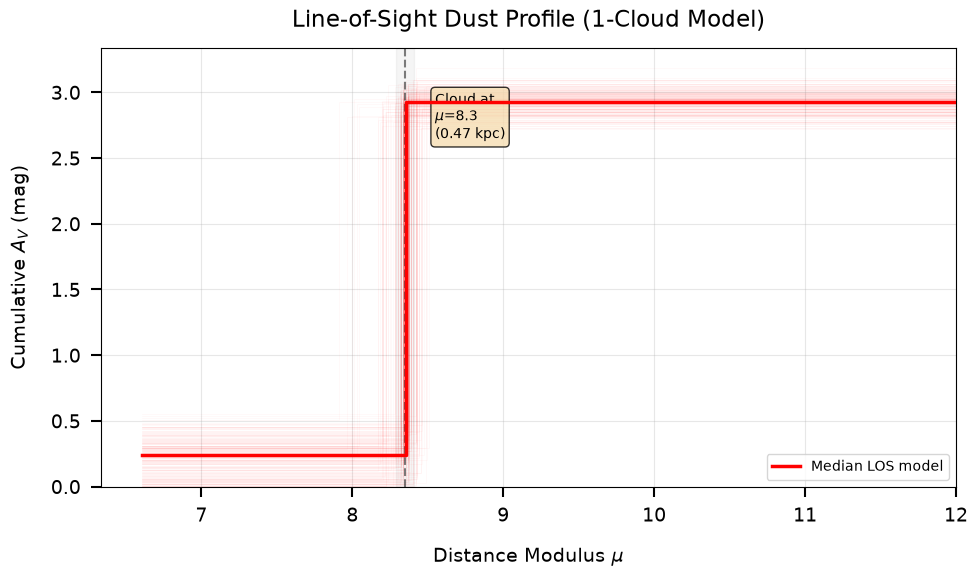
../_images/0688386c621ec39a24559f6596e9cb454e98feb1fb219bc8f3b70615207ea689.png

LOS dust fit visualization complete

Summary and Key Takeaways#

This tutorial has demonstrated line-of-sight dust modeling with brutus:

Key Concepts#

LOS Dust Modeling (brutus.analysis.los_dust)
- Multi-cloud models fit discrete dust structures along the line of sight
- Prior transform + log-likelihood designed for nested sampling (dynesty)
- Compare evidence (logZ) across models with different numbers of clouds. With the default monotonic=True, non-monotone profiles are rejected in the likelihood, shrinking the sampled prior volume, so add back the mode-dependent offset — ln((n+1)!) for an $n$-cloud fit in the default mode — to each logZ before comparing (see the los_clouds_loglike_samples documentation)
Stellar Posteriors
- Per-star distance and extinction samples trace the distance-reddening relation
- bin_pdfs_distred bins and smooths posteriors for visualization

Next Steps#

Tutorial 8: Photometric Calibration
Try fitting 2-cloud and 3-cloud models and comparing evidence (with the ln((n+1)!) offsets noted above)
Apply LOS fitting across multiple sightlines for a 3D dust map

print("Tutorial 7 Complete!")
print("=" * 60)
print("\nGenerated plots:")
for plot_file in sorted(plots_dir.glob('*.png')):
    print(f"  - {plot_file.name}")

Tutorial 7 Complete!
============================================================

Generated plots:
  - dust_sightlines.png
  - kernel_comparison.png
  - los_dust_fit.png
  - stellar_samples.png