Tutorial 10: Plotting Functions

This tutorial provides a standalone demonstration of the main plotting functions in brutus.plotting. The module contains functions for visualizing posterior distributions, SEDs, photometric offsets, and binned distance-reddening PDFs.

Functions Covered

Function	Module	Description
dist_vs_red	brutus.plotting.distance	Distance vs reddening posterior plot
bin_pdfs_distred	brutus.plotting.binning	Bin distance-reddening posterior PDFs
cornerplot	brutus.plotting.corner	Corner plot of multi-dimensional posteriors
posterior_predictive	brutus.plotting.sed	Posterior predictive SED violin plot
photometric_offsets	brutus.plotting.offsets	1-D photometric offset residuals

Note: hist2d from brutus.plotting.utils is the low-level 2-D density histogram utility used internally by cornerplot. It is not demonstrated separately here but can be called directly for custom 2-D density plots.

Prerequisites

• All sections use pre-computed BruteForce results from Orion_l209.1_b-19.9_mist.h5 and optionally the input photometry Orion_l209.1_b-19.9.h5. If these are not available the cells print a skip message.

# Setup: imports and plot style
import warnings

import numpy as np
import matplotlib.pyplot as plt

warnings.filterwarnings("ignore")

# Tutorial utilities
from tutorial_utils import (
    setup_tutorial,
    save_figure,
    print_section,
    find_brutus_data_file,
    load_example_results,
)

# Run the standardized tutorial bootstrap
info = setup_tutorial(10, title="Tutorial 10: Plotting Functions")

# Matplotlib defaults for this notebook
plt.rcParams["figure.figsize"] = (10, 6)

Tutorial 10: Plotting Functions
===============================

Checking data requirements for Tutorial 10
==========================================
  Found: Orion_l204.7_b-19.2_mist.h5

  All required files available

# ---------------------------------------------------------------
# Load pre-computed BruteForce results, input photometry, and models
# ---------------------------------------------------------------
import h5py
from brutus.utils import inv_magnitude
from brutus.data import load_models

DATA_AVAILABLE = False
PHOT_AVAILABLE = False
MODELS_AVAILABLE = False

# Filter names used in the Orion fitting run (PS1 grizy + 2MASS JHKs)
FILTER_NAMES = ['PS_g', 'PS_r', 'PS_i', 'PS_z', 'PS_y',
                '2MASS_J', '2MASS_H', '2MASS_Ks']
N_OBJ_RESULTS = None

# 1. Load BruteForce results
try:
    results = load_example_results("Orion_l209.1_b-19.9_mist.h5")
    DATA_AVAILABLE = True
    N_OBJ_RESULTS = results["model_idx"].shape[0]
    n_samps = results["model_idx"].shape[1]
    print("Loaded BruteForce results.")
    print(f"  File      : {results['filename']}")
    print(f"  Objects   : {N_OBJ_RESULTS}")
    print(f"  Samples   : {n_samps}")
    for key in sorted(results):
        if key == "filename":
            continue
        arr = results[key]
        if isinstance(arr, np.ndarray):
            print(f"  {key:15s}  shape={str(arr.shape):20s}  dtype={arr.dtype}")
except FileNotFoundError as exc:
    print(f"Results file not found -- sections that need it will be skipped.")
    print(f"  ({exc})")

# 2. Load input photometry (subset to match results)
try:
    phot_path = find_brutus_data_file("Orion_l209.1_b-19.9.h5")
    with h5py.File(phot_path, "r") as f:
        fpix = f["photometry"]["pixel 0-0"]
        mag_all = fpix["mag"][:]
        magerr_all = fpix["err"][:]
        plx_all = fpix["parallax"][:]  # already in mas
        plx_err_all = fpix["parallax_error"][:]
        coords_all = np.c_[fpix["l"][:], fpix["b"][:]]

    # Convert to flux
    flux_all, flux_err_all = inv_magnitude(mag_all, magerr_all)
    mask_all = np.isfinite(magerr_all)

    # Subset to match results objects (first N)
    n_sub = N_OBJ_RESULTS if N_OBJ_RESULTS is not None else flux_all.shape[0]
    phot_flux = flux_all[:n_sub]
    phot_flux_err = flux_err_all[:n_sub]
    phot_mask = mask_all[:n_sub]
    phot_parallax = plx_all[:n_sub]
    phot_parallax_err = plx_err_all[:n_sub]
    phot_coords = coords_all[:n_sub]

    PHOT_AVAILABLE = True
    print(f"\nLoaded input photometry from {phot_path}")
    print(f"  Total objects  : {flux_all.shape[0]}")
    print(f"  Subset matched : {n_sub}")
    print(f"  Filters        : {flux_all.shape[1]}")
except FileNotFoundError as exc:
    print(f"\nInput photometry not found (optional).")
    print(f"  ({exc})")

# 3. Load model grid (needed for SED, cornerplot, and offset plots)
try:
    grid_path = find_brutus_data_file("grid_mist_v9.h5")
    models, grid_labels, label_mask = load_models(grid_path, filters=FILTER_NAMES)
    MODELS_AVAILABLE = True
    print(f"\nLoaded model grid from {grid_path}")
    print(f"  models shape  : {models.shape}  (Nmodels, Nfilt, Ncoeff)")
    print(f"  labels shape  : {grid_labels.shape}")
    print(f"  labels fields : {list(grid_labels.dtype.names)}")
except FileNotFoundError as exc:
    print(f"\nModel grid not found.")
    print(f"  ({exc})")

Loaded BruteForce results.
  File      : /mnt/c/Users/joshs/Dropbox/GitHub/brutus/tutorials/Orion_l204.7_b-19.2_mist.h5
  Objects   : 50
  Samples   : 250
  labels           shape=(50,)                 dtype=uint64
  ml_av            shape=(50, 250)             dtype=float32
  ml_cov_sar       shape=(50, 250, 3, 3)       dtype=float32
  ml_rv            shape=(50, 250)             dtype=float32
  ml_scale         shape=(50, 250)             dtype=float32
  model_idx        shape=(50, 250)             dtype=int32
  obj_Nbands       shape=(50,)                 dtype=int16
  obj_chi2min      shape=(50,)                 dtype=float32
  obj_log_evid     shape=(50,)                 dtype=float32
  obj_log_post     shape=(50, 250)             dtype=float32
  samps_dist       shape=(50, 250)             dtype=float32
  samps_dred       shape=(50, 250)             dtype=float32
  samps_logp       shape=(50, 250)             dtype=float32
  samps_red        shape=(50, 250)             dtype=float32

Loaded input photometry from /mnt/c/Users/joshs/Dropbox/GitHub/brutus/tutorials/Orion_l204.7_b-19.2.h5
  Total objects  : 1642
  Subset matched : 50
  Filters        : 8

Reading entire dataset (49 filters) once...

Extracting 8 requested filters from memory...

Loaded model grid from /home/joshspeagle/.cache/astro-brutus/grid_mist_v9.h5
  models shape  : (613530, 8, 3)  (Nmodels, Nfilt, Ncoeff)
  labels shape  : (613530,)
  labels fields : ['mini', 'feh', 'eep', 'loga', 'logl', 'logt', 'logg', 'agewt']

---

Section 2: Distance-Extinction Visualization

This section demonstrates two closely related functions for visualizing distance-extinction posteriors:

• dist_vs_red creates a publication-ready 2-D density image of the joint distance-reddening posterior for a single object.

• bin_pdfs_distred is the data-preparation workhorse behind dist_vs_red. It bins raw BruteForce outputs for multiple objects into 2-D PDFs over the distance-reddening plane.

dist_vs_red Signature

dist_vs_red(data, ebv=None, dist_type='distance_modulus', lndistprior=None,
            coord=None, avlim=(0., 6.), rvlim=(1., 8.), weights=None,
            parallax=None, parallax_err=None, Nr=300, cmap='Blues',
            bins=300, span=None, smooth=0.015, plot_kwargs=None,
            truths=None, truth_color='red', truth_kwargs=None, rstate=None)

data is a 4-tuple (scales, avs, rvs, covs_sar) – the raw per-model BruteForce outputs – or a 3-tuple (dists, reds, dreds) of pre-drawn samples. The function also needs Galactic coordinates (coord) and parallax information when regenerating distance samples from the 4-tuple format.

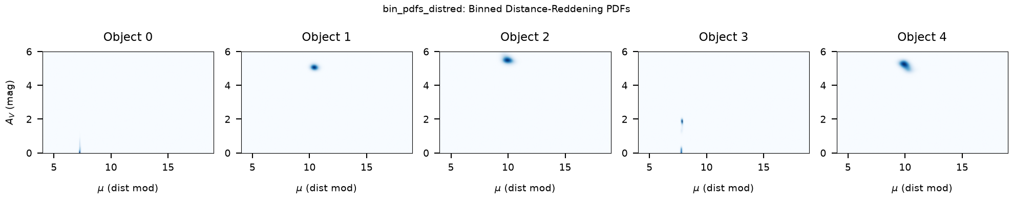
bin_pdfs_distred Signature

bin_pdfs_distred(
    data,           # 4-tuple (scales, avs, rvs, covs_sar) or 3-tuple
    cdf=False, ebv=False, dist_type='distance_modulus',
    lndistprior=None, coord=None, avlim=(0., 6.), rvlim=(1., 8.),
    parallaxes=None, parallax_errors=None, Nr=100,
    bins=(750, 300), span=None, smooth=0.01, rstate=None, verbose=False,
)

Returns (binned_vals, xedges, yedges) where binned_vals has shape (Nobj, Nxbin, Nybin).

Show code cell source

Hide code cell source

from brutus.plotting import dist_vs_red

print_section("2a. dist_vs_red")

if not DATA_AVAILABLE:
    print("SKIPPED -- results file not available.")
else:
    # Pick the first object as an example
    idx = 0

    # Build the 4-tuple that dist_vs_red expects (scale, Av, Rv, cov_sar)
    data_tuple = (
        results["ml_scale"][idx],
        results["ml_av"][idx],
        results["ml_rv"][idx],
        results["ml_cov_sar"][idx],
    )

    # Galactic coordinates for the distance prior
    coord = tuple(phot_coords[idx]) if PHOT_AVAILABLE else (209.1, -19.9)

    # Parallax
    plx = phot_parallax[idx] if PHOT_AVAILABLE else None
    plx_err = phot_parallax_err[idx] if PHOT_AVAILABLE else None

    fig = plt.figure(figsize=(8, 6))
    H, xedges, yedges, img = dist_vs_red(
        data_tuple,
        coord=coord,
        parallax=plx,
        parallax_err=plx_err,
        dist_type="distance_modulus",
        cmap="Blues",
        smooth=0.015,
        bins=300,
    )
    plt.title(f"Object {idx}: Distance Modulus vs A_V")
    plt.colorbar(img, label="Density")

    save_figure(fig, 10, "dist_vs_red_demo")
    plt.show()

    print(f"\nPlotted object {idx}.")
    print(f"  Binned histogram shape : {H.shape}")
    print(f"  Distance modulus range : [{xedges[0]:.1f}, {xedges[-1]:.1f}]")
    print(f"  A_V range              : [{yedges[0]:.1f}, {yedges[-1]:.1f}]")

2a. dist_vs_red
===============

  Saved: /mnt/c/Users/joshs/Dropbox/GitHub/brutus/tutorials/plots/tutorial_10/dist_vs_red_demo.png

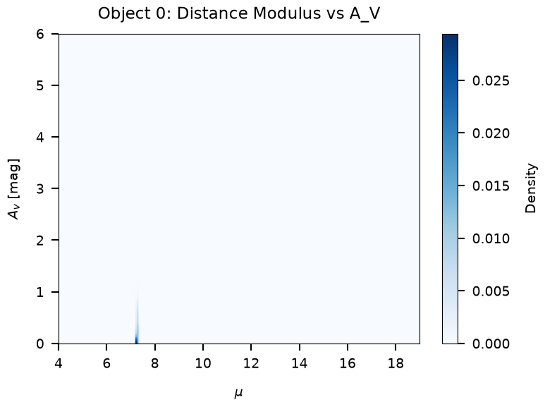
Plotted object 0.
  Binned histogram shape : (300, 300)
  Distance modulus range : [4.0, 19.0]
  A_V range              : [0.0, 6.0]

Binning Distance-Reddening PDFs with bin_pdfs_distred

bin_pdfs_distred operates on multiple objects simultaneously and returns the raw binned arrays, which can be further processed or visualized directly.

Show code cell source

Hide code cell source

from brutus.plotting import bin_pdfs_distred

print_section("2b. bin_pdfs_distred")

if not DATA_AVAILABLE:
    print("SKIPPED -- results file not available.")
else:
    # Use a small subset of objects to keep runtime short
    n_demo = min(5, results["ml_scale"].shape[0])

    data_tuple = (
        results["ml_scale"][:n_demo],
        results["ml_av"][:n_demo],
        results["ml_rv"][:n_demo],
        results["ml_cov_sar"][:n_demo],
    )

    # Coordinates for the distance prior
    if PHOT_AVAILABLE:
        coords_demo = [tuple(c) for c in phot_coords[:n_demo]]
    else:
        coords_demo = [(209.1, -19.9)] * n_demo

    plx_demo = phot_parallax[:n_demo] if PHOT_AVAILABLE else None
    plx_err_demo = phot_parallax_err[:n_demo] if PHOT_AVAILABLE else None

    binned_vals, xedges, yedges = bin_pdfs_distred(
        data_tuple,
        coord=coords_demo,
        parallaxes=plx_demo,
        parallax_errors=plx_err_demo,
        bins=(200, 100),
        smooth=0.015,
        verbose=True,
    )
    print()  # newline after progress output

    print(f"\nbinned_vals shape : {binned_vals.shape}  (Nobj, Nxbin, Nybin)")
    print(f"xedges shape      : {xedges.shape}")
    print(f"yedges shape      : {yedges.shape}")

    # Visualise the binned PDFs for each object
    fig, axes = plt.subplots(1, n_demo, figsize=(4 * n_demo, 4), squeeze=False)
    for i in range(n_demo):
        ax = axes[0, i]
        ax.imshow(
            binned_vals[i].T,
            origin="lower",
            aspect="auto",
            extent=[xedges[0], xedges[-1], yedges[0], yedges[-1]],
            cmap="Blues",
        )
        ax.set_xlabel(r"$\mu$ (dist mod)")
        if i == 0:
            ax.set_ylabel(r"$A_V$ (mag)")
        ax.set_title(f"Object {i}")

    plt.suptitle("bin_pdfs_distred: Binned Distance-Reddening PDFs", fontsize=14)
    save_figure(fig, 10, "bin_pdfs_distred_demo")
    plt.show()

    print(f"\nPlotted {n_demo} objects.")

2b. bin_pdfs_distred
====================

binned_vals shape : (5, 200, 100)  (Nobj, Nxbin, Nybin)
xedges shape      : (201,)
yedges shape      : (101,)

Binning object 1/5
Binning object 2/5
Binning object 3/5
Binning object 4/5
Binning object 5/5

  Saved: /mnt/c/Users/joshs/Dropbox/GitHub/brutus/tutorials/plots/tutorial_10/bin_pdfs_distred_demo.png

Plotted 5 objects.

---

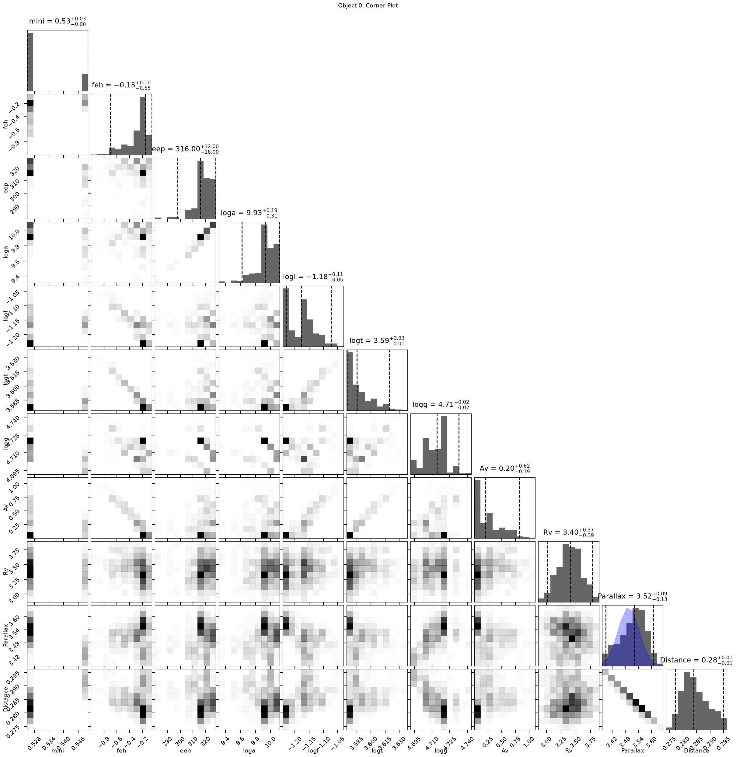
Section 3: cornerplot – Corner Plot of Posteriors

cornerplot generates a corner plot showing 1-D and 2-D marginalized posteriors for all stellar parameters (from the model grid labels) plus A_V, R_V, parallax, and distance.

Signature

cornerplot(idxs, data, params,
           lndistprior=None, coord=None, avlim=(0., 6.), rvlim=(1., 8.),
           weights=None, parallax=None, parallax_err=None, Nr=500,
           applied_parallax=True, pcolor='blue', parallax_kwargs=None,
           span=None, quantiles=[0.025, 0.5, 0.975], color='black',
           smooth=10, hist_kwargs=None, hist2d_kwargs=None, labels=None,
           label_kwargs=None, show_titles=False, title_fmt='.2f',
           title_kwargs=None, title_quantiles=[0.025, 0.5, 0.975],
           truths=None, truth_color='red', truth_kwargs=None,
           max_n_ticks=5, top_ticks=False, use_math_text=False,
           verbose=False, fig=None, rstate=None)

Required inputs:

• idxs – resampled model indices (shape (Nsamps,)).

• data – 4-tuple (scales, avs, rvs, covs_sar) or 3-tuple (dists, reds, dreds).

• params – structured array of model parameters (from the grid via load_models).

Show code cell source

Hide code cell source

from brutus.plotting import cornerplot

print_section("Section 3: cornerplot")

if DATA_AVAILABLE and MODELS_AVAILABLE:
    idx = 0

    idxs_obj = results["model_idx"][idx]
    data_tuple = (
        results["ml_scale"][idx],
        results["ml_av"][idx],
        results["ml_rv"][idx],
        results["ml_cov_sar"][idx],
    )

    coord = tuple(phot_coords[idx]) if PHOT_AVAILABLE else (209.1, -19.9)
    plx = phot_parallax[idx] if PHOT_AVAILABLE else None
    plx_err = phot_parallax_err[idx] if PHOT_AVAILABLE else None

    fig, axes = cornerplot(
        idxs_obj,
        data_tuple,
        grid_labels,
        coord=coord,
        parallax=plx,
        parallax_err=plx_err,
        applied_parallax=(plx is not None),
        smooth=10,
        show_titles=True,
        verbose=True,
    )
    fig.suptitle(f"Object {idx}: Corner Plot", y=1.02, fontsize=14)

    save_figure(fig, 10, "cornerplot_demo", tight=False)
    plt.show()

    print(f"\nCorner plot has {len(axes)} rows/columns of panels.")
else:
    print("SKIPPED -- need both results file and model grid.")

Section 3: cornerplot
=====================

Quantiles:
mini [(0.025, np.float64(0.8750000000000003)), (0.5, np.float64(1.0500000000000005)), (0.975, np.float64(1.2750000000000008))]
Quantiles:
feh [(0.025, np.float64(-0.7124999999999988)), (0.5, np.float64(-0.09999999999999831)), (0.975, np.float64(0.30000000000000204))]
Quantiles:
eep [(0.025, np.float64(370.0)), (0.5, np.float64(442.0)), (0.975, np.float64(456.0))]
Quantiles:
loga [(0.025, np.float64(9.465241338009797)), (0.5, np.float64(9.849791395117133)), (0.975, np.float64(10.051082153372834))]
Quantiles:
logl [(0.025, np.float64(0.329651589183751)), (0.5, np.float64(0.4285395918453292)), (0.975, np.float64(0.5248467949096491))]
Quantiles:
logt [(0.025, np.float64(3.749565228908653)), (0.5, np.float64(3.776680532855328)), (0.975, np.float64(3.8054007333187183))]
Quantiles:
logg [(0.025, np.float64(3.9980454611166354)), (0.5, np.float64(4.098561191383948)), (0.975, np.float64(4.221587716143503))]
Quantiles:
Av [(0.025, np.float64(0.6382905893614429)), (0.5, np.float64(0.883455461596611)), (0.975, np.float64(1.1264052628693069))]
Quantiles:
Rv [(0.025, np.float64(3.092424263434222)), (0.5, np.float64(3.2996664171917347)), (0.975, np.float64(3.4861411211118645))]

Quantiles:
Parallax [(0.025, np.float64(1.0108323735055544)), (0.5, np.float64(1.0700351463781272)), (0.975, np.float64(1.1269807405509698))]
Quantiles:
Distance [(0.025, np.float64(0.8873269541492314)), (0.5, np.float64(0.9345487533514693)), (0.975, np.float64(0.9892837139704419))]

  Saved: /mnt/c/Users/joshs/Dropbox/GitHub/brutus/tutorials/plots/tutorial_10/cornerplot_demo.png

Corner plot has 11 rows/columns of panels.

---

Section 4: posterior_predictive – SED Posterior Predictive Plot

posterior_predictive shows the predicted SED (as violin plots across filters) compared with observed photometry. It uses the model polynomial coefficients array (models) and pre-computed posterior samples (model_idx, samps_red, samps_dred, samps_dist) from BruteForce output.

Signature

posterior_predictive(models, idxs, reds, dreds, dists,
                     weights=None, flux=False,
                     data=None, data_err=None, data_mask=None,
                     offset=None, vcolor='black', pcolor='black',
                     labels=None, rstate=None, psig=2., fig=None)

Show code cell source

Hide code cell source

from brutus.plotting import posterior_predictive

print_section("Section 4: posterior_predictive")

if DATA_AVAILABLE and MODELS_AVAILABLE:
    idx = 0

    # Use pre-computed posterior samples directly from BruteForce output
    idxs_obj = results["model_idx"][idx]
    reds_obj = results["samps_red"][idx]      # A_V samples
    dreds_obj = results["samps_dred"][idx]    # R_V samples
    dists_obj = results["samps_dist"][idx]    # distance in kpc

    # Observed photometry for overplot
    obs_flux = phot_flux[idx] if PHOT_AVAILABLE else None
    obs_err = phot_flux_err[idx] if PHOT_AVAILABLE else None
    obs_mask = phot_mask[idx] if PHOT_AVAILABLE else None

    fig, ax, parts = posterior_predictive(
        models,
        idxs_obj,
        reds_obj,
        dreds_obj,
        dists_obj,
        data=obs_flux,
        data_err=obs_err,
        data_mask=obs_mask,
        labels=FILTER_NAMES,
        vcolor="steelblue",
        pcolor="red",
    )
    ax.set_title(f"Object {idx}: Posterior Predictive SED")

    save_figure(fig, 10, "posterior_predictive_demo")
    plt.show()

    print(f"\nViolin bodies plotted across {len(FILTER_NAMES)} filters.")
else:
    print("SKIPPED -- need both results file and model grid.")

Section 4: posterior_predictive
===============================

  Saved: /mnt/c/Users/joshs/Dropbox/GitHub/brutus/tutorials/plots/tutorial_10/posterior_predictive_demo.png

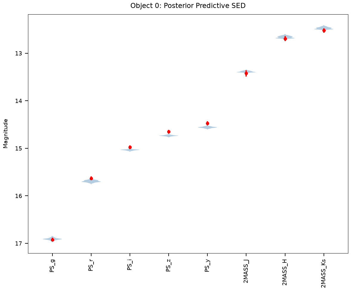
Violin bodies plotted across 8 filters.

---

Section 5: photometric_offsets – 1-D Offset Residuals

photometric_offsets computes mag_pred - mag_obs for every band and plots the residual as a function of observed magnitude. Each panel corresponds to one photometric filter. This is a diagnostic tool for identifying systematic model-data discrepancies as a function of brightness.

Note: this is a plotting function (brutus.plotting.offsets), distinct from the analysis function of the same name (brutus.analysis.offsets) demonstrated in Tutorial 8. The analysis function computes multiplicative calibration corrections; this function visualizes magnitude residuals.

Signature

photometric_offsets(
    phot, err, mask, models, idxs, reds, dreds, dists,
    x=None, flux=True, weights=None, bins=100,
    offset=None, dim_prior=True, plot_thresh=0.,
    cmap='viridis', xspan=None, yspan=None,
    titles=None, xlabel=None, plot_kwargs=None, fig=None,
)

Show code cell source

Hide code cell source

from brutus.plotting import photometric_offsets as plot_phot_offsets

print_section("Section 5: photometric_offsets")

if DATA_AVAILABLE and MODELS_AVAILABLE and PHOT_AVAILABLE:
    # Use all 50 fitted objects with their posterior samples
    fig, axes = plot_phot_offsets(
        phot_flux,
        phot_flux_err,
        phot_mask,
        models,
        results["model_idx"],
        results["samps_red"],
        results["samps_dred"],
        results["samps_dist"],
        flux=True,
        bins=15,
        titles=FILTER_NAMES,
        cmap="viridis",
    )
    fig.suptitle(
        "Photometric Offset Residuals (model - observed)",
        fontsize=14, y=1.02,
    )

    save_figure(fig, 10, "photometric_offsets_demo", tight=False)
    plt.show()

    print(f"\nPlotted residuals for {len(FILTER_NAMES)} filters "
          f"across {phot_flux.shape[0]} objects.")
else:
    print("SKIPPED -- need results, photometry, and model grid.")

Section 5: photometric_offsets
==============================

  Saved: /mnt/c/Users/joshs/Dropbox/GitHub/brutus/tutorials/plots/tutorial_10/photometric_offsets_demo.png

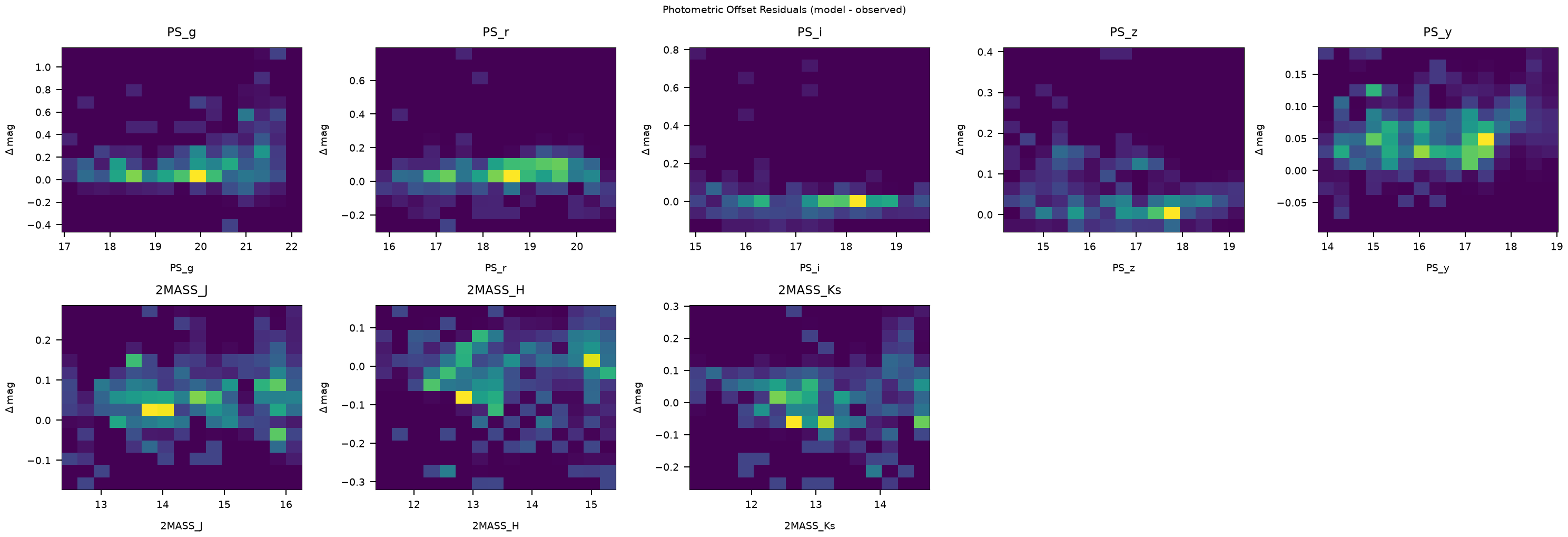
Plotted residuals for 8 filters across 50 objects.

---

Summary

This tutorial demonstrated the main plotting functions in brutus.plotting using real BruteForce results from the Orion sightline (Tutorial 5):

#	Function	Section	Data Used
1	dist_vs_red	Section 1	BruteForce posteriors
2	bin_pdfs_distred	Section 1	BruteForce posteriors
3	cornerplot	Section 2	BruteForce posteriors + grid labels
4	posterior_predictive	Section 3	BruteForce posteriors + grid models
5	photometric_offsets	Section 4	BruteForce posteriors + models + photometry

Key Points

• dist_vs_red and bin_pdfs_distred work together: the latter bins the data and the former wraps it into a publication-ready figure.

• cornerplot gives a full multi-parameter view including stellar labels, A_V, R_V, parallax, and distance. It uses hist2d internally for the off-diagonal 2-D density panels.

• posterior_predictive compares predicted and observed SEDs filter by filter.

• photometric_offsets is a diagnostic visualization tool for identifying systematic model-data residuals. It is distinct from the calibration analysis function of the same name in brutus.analysis.offsets (demonstrated in Tutorial 8).

Related Tutorials

• Tutorial 5 – Fitting Individual Sources (produces the results used here).

• Tutorial 7 – 3D Dust Mapping (uses dist_vs_red and bin_pdfs_distred).

• Tutorial 8 – Photometric Calibration (uses the analysis photometric_offsets function to compute multiplicative corrections).